Artificial intelligence (AI) has been at the forefront of technology over the last few years, and has made its way into mainstream applications, such as expert systems, personalized applications on mobile devices, machine translation in natural language processing, chatbots, self-driving cars, and so on. The definition of AI, however, has been a subject of dispute for quite a while. This is primarily because of the so-called AI effect that categorizes work that has already been solved through AI in the past as non-AI. According to a famous computer scientist:

Building an intelligent system that could play chess was considered AI until the IBM computer Deep Blue defeated Gary Kasparov in 1996. Similarly, problems dealing with vision, speech, and natural language were once considered complex, but due to the AI effect, they would now only be considered computation rather than true AI. Recently, AI has become able to solve complex mathematical problems, compose music, and create abstract paintings, and these capabilities of AI are ever increasing. The point in the future at which AI systems will equal human levels of intelligence has been referred to by scientists as the AI singularity. The question of whether machines will ever actually reach human levels of intelligence is very intriguing.

Many would argue that machines will never reach human levels of intelligence, since the AI logic by which they learn or perform intelligent tasks is programmed by humans, and they lack the consciousness and self-awareness that humans possess. However, several researchers have proposed the alternative idea that human consciousness and self-awareness are like infinite loop programs that learn from their surroundings through feedback. Hence, it may be possible to program consciousness and self-awareness into machines, too. For now, however, we will leave this philosophical side of AI for another day, and will simply discuss AI as we know it.

Put simply, AI can be defined as the ability of a machine (generally, a computer or robot) to perform tasks with human-like intelligence, possessing such as attributes the ability to reason, learn from experience, generalize, decipher meanings, and possess visual perception. We will stick to this more practical definition rather than looking at the philosophical connotations raised by the AI effect and the prospect of the AI singularity. While there may be debates about what AI can achieve and what it cannot, recent success stories of AI-based systems have been overwhelming. A few of the more recent mainstream applications of AI are depicted in the following diagram:

This book will cover the detailed implementation of projects from all of the core disciplines of AI, outlined as follows:

• Transfer learning based AI systems
• Natural language based AI systems
• Generative adversarial network (GAN) based applications
• Expert systems
• Video-to-text translation applications
• AI-based recommender systems
• AI-based mobile applications
• AI-based chatbots
• Reinforcement learning applications

In this chapter, we will briefly touch upon the concepts involving machine learning and deep learning that will be required to implement the projects that will be covered in the following chapters.

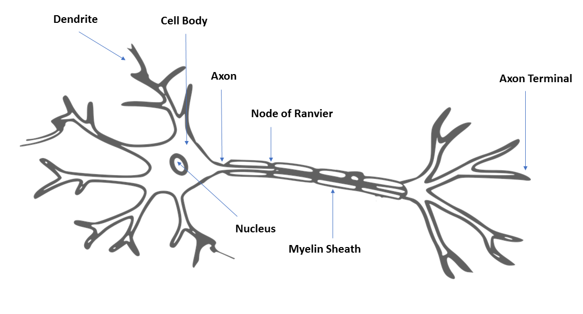
Neural networks are machine learning models that are inspired by the human brain. They consist of neural processing units they are interconnected with one another in a hierarchical fashion. These neural processing units are called artificial neurons, and they perform the same function as axons in a human brain. In a human brain, dendrites receive input from neighboring neurons, and attenuate or magnify the input before transmitting it on to the soma of the neuron. In the soma of the neuron, these modified signals are added together and passed on to the axon of the neuron. If the input to the axon is over a specified threshold, then the signal is passed on to the dendrites of the neighboring neurons.

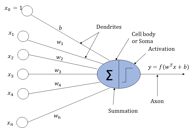
An artificial neuron loosely works perhaps on the same logic as that of a biological neuron. It receives input from neighboring neurons. The input is scaled by the input connections of the neurons and then added together. Finally, the summed input is passed through an activation function whose output is passed on to the neurons in the next layer.

A biological neuron and an artificial neuron are illustrated in the following diagrams for comparison:

An artificial neuron are illustrated in the following diagram:

Now, let's look at the structure of an artificial neural network, as illustrated in the following diagram:

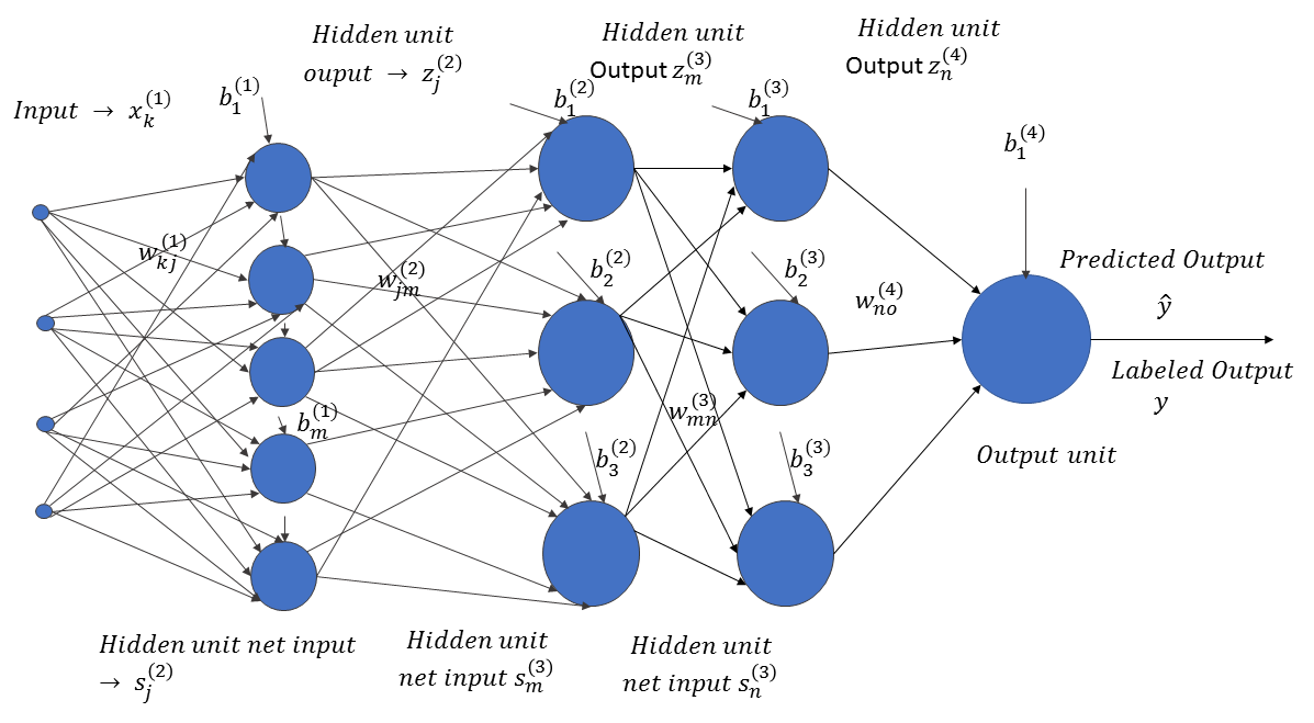
The input, x ∈ R^N, passes through successive layers of neural units, arranged in a hierarchical fashion. Each neuron in a specific layer receives an input from the neurons of the preceding layers, attenuated or amplified by the weights of the connections between them. The weight, , corresponds to the weight connection between the i^th neuron in layer l and the j^th neuron in layer (l+1). Also, each neuron unit, i, in a specific layer, l, is accompanied by a bias, . The neural network predicts the output, , for the input vector, x ∈ R^N. If the actual label of the data is y, where y takes continuous values, then the neuron network learns the weights and biases by minimizing the prediction error, . Of course, the error has to be minimized for all of the labeled data points: (x_i, y_i)∀_i ∈ 1, 2, . . . m.

If we denote the set of weights and biases by one common vector, W, and the total error in the prediction is represented by C, then through the training process, the estimated W can be expressed as follows:

Also, the predicted output, , can be represented by a function of the input, x, parameterized by the weight vector, W, as follows:

Such a formula for predicting the continuous values of the output is called a regression problem.

For a two-class binary classification, cross-entropy loss is minimized instead of the squared error loss, and the network outputs the probability of the positive class instead of the output. The cross-entropy loss can be represented as follows:

Here, p_i is the predicted probability of the output class, given the input x, and can be represented as a function of the input, x, parameterized by the weight vector, as follows:

In general, for multi-class classification problems (say, of n classes), the cross-entropy loss is given via the following:

Here, is the output label of the j^th class, for the i^th datapoint.

Several kinds of neural activation units are used in neural networks, depending on the architecture and the problem at hand. We will discuss the most commonly used activation functions, as these play an important role in determining the network architecture and performance. Linear and sigmoid unit activation functions were primarily used in artificial neural networks until rectified linear units (ReLUs), invented by Hinton et al., revolutionized the performance of neural networks.

A linear activation unit outputs the total input to the neuron that is attenuated, as shown in the following graph:

If x is the total input to the linear activation unit, then the output, y, can be represented as follows:

The output of the sigmoid activation unit, y, as a function of its total input, x, is expressed as follows:

Since the sigmoid activation unit response is a nonlinear function, as shown in the following graph, it is used to introduce nonlinearity in the neural network:

Any complex process in nature is generally nonlinear in its input-output relation, and hence, we need nonlinear activation functions to model them through neural networks. The output probability of a neural network for a two-class classification is generally given by the output of a sigmoid neural unit, since it outputs values from zero to one. The output probability can be represented as follows:

Here, x represents the total input to the sigmoid unit in the output layer.

The output, y, of a hyperbolic tangent activation function (tanh) as a function of its total input, x, is given as follows:

The tanh activation function outputs values in the range [-1, 1], as you can see in the following graph:

One thing to note is that both the sigmoid and the tanh activation functions are linear within a small range of the input, beyond which the output saturates. In the saturation zone, the gradients of the activation functions (with respect to the input) are very small or close to zero; this means that they are very prone to the vanishing gradient problem. As you will see later on, neural networks learn from the backpropagation method, where the gradient of a layer is dependent on the gradients of the activation units in the succeeding layers, up to the final output layer. Therefore, if the units in the activation units are working in the saturation region, much less of the error is backpropagated to the early layers of the neural network. Neural networks minimize the prediction error in order to learn the weights and biases (W) by utilizing the gradients. This means that, if the gradients are small or vanish to zero, then the neural network will fail to learn these weights properly.

The output of a ReLU is linear when the total input to the neuron is greater than zero, and the output is zero when the total input to the neuron is negative. This simple activation function provides nonlinearity to a neural network, and, at the same time, it provides a constant gradient of one with respect to the total input. This constant gradient helps to keep the neural network from developing saturating or vanishing gradient problems, as seen in activation functions, such as sigmoid and tanh activation units. The ReLU function output (as shown in Figure 1.8) can be expressed as follows:

The ReLU activation function can be plotted as follows:

One of the constraints for ReLU is its zero gradients for negative values of input. This may slow down the training, especially at the initial phase. Leaky ReLU activation functions (as shown in Figure 1.9) can be useful in this scenario, where the output and gradients are nonzero, even for negative values of the input. A leaky ReLU output function can be expressed as follows:

The parameter is to be provided for leaky ReLU activation functions, whereas for a parametric ReLU, is a parameter that the neural network will learn through training. The following graph shows the output of the leaky ReLU activation function:

The softmax activation unit is generally used to output the class probabilities, in the case of a multi-class classification problem. Suppose that we are dealing with an n class classification problem, and the total input corresponding to the classes is given by the following:

In this case, the output probability of the k^th class of the softmax activation unit is given by the following formula:

There are several other activation functions, mostly variations of these basic versions. We will discuss them as we encounter them in the different projects that we will cover in the following chapters.

In the backpropagation method, neural networks are trained through the gradient descent technique, where the combined weights vector, W, is updated iteratively, as follows:

Here, η is the learning rate, W^(t+1) and W^(t) are the weight vectors at iterations (t+1) and (t), respectively, and ∇C(W^(t)) is the gradient of the cost function or the error function, with respect to the weight vector, W, at iteration (t). The previous algorithm for an individual weight or bias generalized by w ∈ W can be represented as follows:

As you can gather from the previous expressions, the heart of the gradient descent method of learning relies on computing the gradient of the cost function or the error function, with respect to each weight.

From the chain rule of differentiation, we know that if we have y = f(x), z = f(y), then the following is true:

This expression can be generalized to any number of variables. Now, let's take a look at a very simple neural network, as illustrated in the following diagram, in order to understand the backpropagation algorithm:

Let the input to the network be a two-dimensional vector, x = [x₁ x₂]^T, and the corresponding output label and prediction be and , respectively. Also, let's assume that all of the activation units in the neural network are sigmoids. Let the generalized weight connecting any unit i in layer (l-1) to unit j in layer l be denoted by , while the bias in any unit i in layer l should be denoted by . Let's derive the gradient for one data point; the total gradient can be computed as the sum of all of the data points used in training (or in a mini-batch). If the output is continuous, then the loss function, C, can be chosen as the square of the error in prediction:

The weights and biases of the network, cumulatively represented by the set W, can be determined by minimizing the cost function with respect to the W vector, which is as follows:

To perform the minimization of the cost function iteratively through gradient descent, we need to compute the gradient of the cost function with respect to each weight, w ∈ W, as follows:

Now that we have everything that we need, let's compute the gradient of the cost function, C, with respect to the weight, . Using the chain rule of differentiation, we get the following:

Now let's look at the following formula:

As you can see in the previous expression, the derivative is nothing but the error in prediction. Generally, the output unit activation function is linear in the case of regression problems, and hence the following expression applies:

So, if we were to compute the gradient of the cost function with respect to the total input at the output unit, it would be . This is still equal to the error in prediction of the output.

The total input at the output unit, as a function of the incoming weights and activations, can be expressed as follows:

This means that, and the derivative of the cost function with respect to the weight, , contributing to the input of the output layer is given via the following:

As you can see, the error is backpropagated in computing the gradient of the cost function, with respect to the weights in the layers preceding the final output layer. This becomes more obvious when we compute the gradient of the cost function with respect to the generalized weight, . Let's take the weight corresponding to j=1 and k=2; that is, . The gradient of the cost function, C, with respect to this weight can be expressed as follows:

Now, , which means that, .

So, once we have figured out the gradient of the cost function with respect to the total input to a neuron as , the gradient of any weight, w, contributing to the total input, s, can be obtained by simply multiplying the activation, z, associated with the weight.

Now, the gradient of the cost function with respect to the total input, , can be derived by chain rule again, as follows:

Since all of the units of the neural network (except for the output unit) are sigmoid activation functions, the following is the case:

Combining (1), (2), and (3), we get the following:

In the preceding derived gradient expressions, you can see that the error in prediction, , is backpropagated by combining it with the relevant activations and weights (as per the chain rule of differentiation) for computing the gradients of the weights at each layer, hence, the name backpropagation in AI nomenclature.

Convolutional neural networks (CNNs) utilize convolutional operations to extract useful information from data that has a topology associated with it. This works best for image and audio data. The input image, when passed through a convolution layer, produces several output images, known as output feature maps. The output feature maps detect features. The output feature maps in the initial convolutional layer may learn to detect basic features, such as edges and color composition variation.

The second convolutional layer may detect slightly more complicated features, such as squares, circles, and other geometrical structures. As we progress through the neural network, the convolutional layers learn to detect more and more complicated features. For instance, if we have a CNN that classifies whether an image is of a cat or a dog, the convolutional layers at the bottom of the neural network might learn to detect features such as the head, the legs, and so on.

Figure 1.11 shows an architectural diagram of a CNN that processes images of cats and dogs in order to classify them. The images are passed through a convolutional layer that helps to detect relevant features, such as edges and color composition. The ReLU activations add nonlinearity. The pooling layer that follows the activation layer summarizes local neighborhood information in order to provide an amount of translational invariance. In an ideal CNN, this convolution-activation-pooling operation is performed several times before the network makes its way to the dense connections:

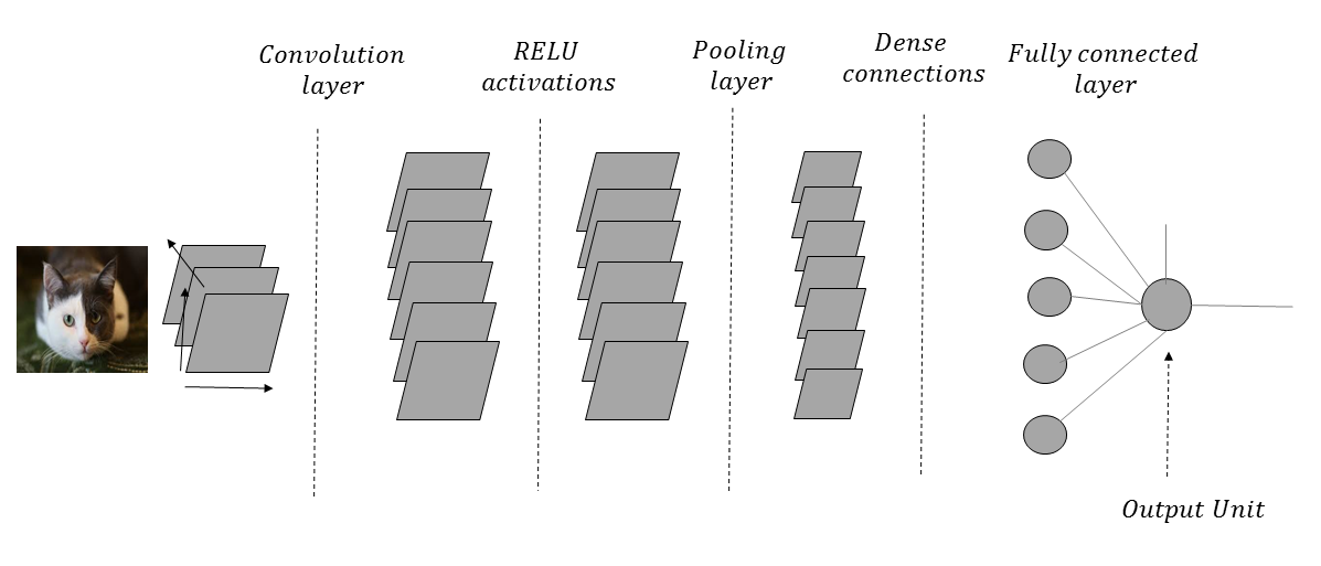
As we go through such a network with several convolution-activation-pooling operations, the spatial resolution of the image is reduced, while the number of output feature maps is increased in every layer. Each output feature map in a convolutional layer is associated with a filter kernel, the weights of which are learned through the CNN training process.

In a convolutional operation, a flipped version of a filter kernel is laid over the entire image or feature map, and the dot product of the filter-kernel input values with the corresponding image pixel or the feature map values are computed for each location on the input image or feature map. Readers that are already accustomed to ordinary image processing may have used different filter kernels, such as a Gaussian filter, a Sobel edge detection filter, and many more, where the weights of the filters are predefined. The advantage of convolutional neural networks is that the different filter weights are determined through the training process; This means that, the filters are better customized for the problem that the convolutional neural network is dealing with.

When a convolutional operation involves overlaying the filter kernel on every location of the input, the convolution is said to have a stride of one. If we choose to skip one location while overlaying the filter kernel, then convolution is performed with a stride of two. In general, if n locations are skipped while overlaying the filter kernel over the input, the convolution is said to have been performed with a stride of (n+1). Strides of greater than one reduce the spatial dimensions of the output of the convolution.

Generally, a convolutional layer is followed by a pooling layer, which basically summarizes the output feature map activations in a neighborhood, determined by the receptive field of the pooling. For instance, a 2 x 2 receptive field will gather the local information of four neighboring output feature map activations. For max-pooling operations, the maximum value of the four activations is selected as the output, while for average pooling, the average of the four activations is selected. Pooling reduces the spatial resolution of the feature maps. For instance, for a 224 x 224 sized feature map pooling operation with a 2 x 2 receptive field, the spatial dimension of the feature map will be reduced to 112 x 112.

One thing to note is that a convolutional operation reduces the number of weights to be learned in each layer. For instance, if we have an input image of a spatial dimension of 224 x 224 and the desired output of the next layer is of the dimensions 224 x 224, then for a traditional neural network with full connections, the number of weights to be learned is 224 x 224 x 224 x 224. For a convolutional layer with the same input and output dimensions, all that we need to learn are the weights of the filter kernel. So, if we use a 3 x 3 filter kernel, we just need to learn nine weights as opposed to 224 x 224 x 224 x 224 weights. This simplification works, since structures like images and audio in a local spatial neighborhood have high correlation among them.

The input images pass through several layers of convolutional and pooling operations. As the network progresses, the number of feature maps increases, while the spatial resolution of the images decreases. At the end of the convolutional-pooling layers, the output of the feature maps is fed to the fully connected layers, followed by the output layer.

The output units are dependent on the task at hand. If we are performing regression, the output activation unit is linear, while if it is a binary classification problem, the output unit is a sigmoid. For multi-class classification, the output layer is a softmax unit.

In all of the image processing projects in this book, we will use convolutional neural networks, in one form or another.

Recurrent neural networks (RNNs) are useful in processing sequential or temporal data, where the data at a given instance or position is highly correlated with the data in the previous time steps or positions. RNNs have already been very successful at processing text data, since a word at a given instance is highly correlated with the words preceding it. In an RNN, at each time step, the network performs the same function, hence, the term recurrent in its name. The architecture of an RNN is illustrated in the following diagram:

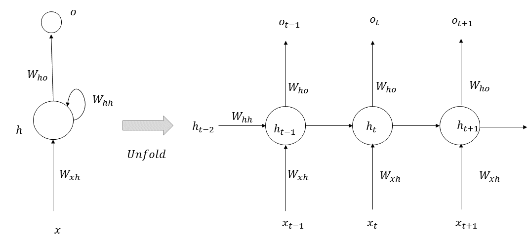
At each given time step, t, a memory state, h_t, is computed, based on the previous state, h_t-1, at step (t-1) and the input, x_t, at time step t. The new state, h_t, is used to predict the output, o_t, at step t. The equations governing RNNs are as follows:

If we are predicting the next word in a sentence, then the function f₂ is generally a softmax function over the words in the vocabulary. The function f₁ can be any activation function based on the problem at hand.

In an RNN, an output error in step t tries to correct the prediction in the previous time steps, generalized by k ∈ 1, 2, . . . t-1, by propagating the error in the previous time steps. This helps the RNN to learn about long dependencies between words that are far apart from each other. In practice, it isn't always possible to learn such long dependencies through RNN because of the vanishing and exploding gradient problems.

As you know, neural networks learn through gradient descent, and the relationship of a word in time step t with a word at a prior sequence step k can be learned through the gradient of the memory state with respect to the gradient of the memory state ∀ i. This is expressed in the following formula:

If the weight connection from the memory state at the sequence step k to the memory state at the sequence step (k+1) is given by u_ii ∈ W_hh, then the following is true:

In the preceding equation, is the total input to the memory state i at the time step (k+1), such that the following is the case:

Now that we have everything in place, it's easy to see why the vanishing gradient problem may occur in an RNN. From the preceding equations, (3) and (4), we get the following:

For RNNs, the function f₂ is generally sigmoid or tanh, which suffers from the saturation problem of having low gradients beyond a specified range of values for the input. Now, since the f₂ derivatives are multiplied with each other, the gradient can become zero if the input to the activation functions is operating at the saturation zone, even for relatively moderate values of (t-k). Even if the f₂ functions are not operating in the saturation zone, the gradients of the f₂ function for sigmoids are always less than 1, and so it is very difficult to learn distant dependencies between words in a sequence. Similarly, there might be exploding gradient problems stemming from the factor . Suppose that the distance between steps t and k is around 10, while the weight, u_ii, is around two. In such cases, the gradient would be magnified by a factor of two, 2¹⁰ = 1024, leading to the exploding gradient problem.

The vanishing gradient problem is taken care of, to a great extent, by a modified version of RNNs, called long short-term memory (LSTM) cells. The architectural diagram of a long short-term memory cell is as follows:

LSTM introduces the cell state, C_t, in addition to the memory state, h_t, that you already saw when learning about RNNs. The cell state is regulated by three gates: the forget gate, the update gate, and the output gate. The forget gate determines how much information to retain from the previous cell states, C_t-1, and its output is expressed as follows:

The output of the update gate is expressed as follows:

The potential new candidate cell state, , is expressed as follows:

Based on the previous cell state and the current potential cell state, the updated cell state output is given via the following:

Not all of the information of the cell state is passed on to the next step, and how much of the cell state should be released to the next step is determined by the output gate. The output of the output gate is given via the following:

Based on the current cell state and the output gate, the updated memory state passed on to the next step is given via the following:

Now comes the big question: How does LSTM avoid the vanishing gradient problem? The equivalent of in LSTM is given by , which can be expressed in a product form as follows:

Now, the recurrence in the cell state units is given by the following:

From this, we get the following:

As a result, the gradient expression, , becomes the following:

As you can see, if we can keep the forget cell state near one, the gradient will flow almost unattenuated, and the LSTM will not suffer from the vanishing gradient problem.

Most of the text-processing applications that we will look at in this book will use the LSTM version of RNNs.

Generative adversarial networks, popularly known as GANs, are generative models that learn a specific probability distribution through a generator, G. The generator G plays a zero sum minimax game with a discriminator D and both evolve over time, before the Nash equilibrium is reached. The generator tries to produce samples similar to the ones generated by a given probability distribution, P(x), while the discriminator D tries to distinguish those fake data samples generated by the generator G from the data sample from the original distribution. The generator G tries to generate samples similar to the ones from P(x), by converting samples, z, drawn from a noise distribution, P(z). The discriminator, D, learns to tag samples generated by the generator G as G(z) when fake; x belongs to P(x) when they are original. At the equilibrium of the minimax game, the generator will learn to produce samples similar to the ones generated by the original distribution, P(x), so that the following is true:

The following diagram illustrates a GAN network learning the probability distribution of the MNIST digits:

The cost function minimized by the discriminator is the binary cross-entropy for distinguishing the real data points belonging to the probability distribution P(x) from the fake ones generated by the generator (that is, G(z)):

The generator will try to maximize the same cost function given by (1). This means that, the optimization problem can be formulated as a minimax player with the utility function U(G,D), as illustrated here:

Generally, to measure how far a given probability distribution matches that of a given distribution, f-divergence measures are used, such as the Kullback–Leibler (KL) divergence, the Jensen Shannon divergence, and the Bhattacharyya distance. For example, the KL divergence between two probability distributions, P and Q, is given by the following, where the expectation is with respect to the distribution, P:

Similarly, the Jensen Shannon divergence between P and Q is given as follows:

Now, coming back to (2), the expression can be written as follows:

Here, G(x) is the probability distribution for the generator. Expanding the expectation into its integral form, we get the following:

For a fixed generator distribution, G(x), the utility function will be at a minimum with respect to the discriminator if the following is true:

Substituting D(x) from (5) in (3), we get the following:

Now, the task of the generator is to maximize the utility, , or minimize the utility, . The expression for can be rearranged as follows:

Hence, we can see that the generator minimizing is equivalent to minimizing the Jensen Shannon divergence between the real distribution, P(x), and the distribution of the samples generated by the generator, G (that is, G(x)).

Training a GAN is not a straightforward process, and there are several technical considerations that we need to take into account while training such a network. We will be using an advanced GAN network to build a cross-domain style transfer application in Chapter 4, Style Transfer in Fashion Industry using GANs.

Reinforcement learning is a branch of machine learning that enables machines and/or agents to maximize some form of reward within a specific context by taking specific actions. Reinforcement learning is different from supervised and unsupervised learning. Reinforcement learning is used extensively in game theory, control systems, robotics, and other emerging areas of artificial intelligence. The following diagram illustrates the interaction between an agent and an environment in a reinforcement learning problem:

We will now look at a popular reinforcement learning algorithm, called Q-learning. Q-learning is used to determine an optimal action selection policy for a given finite Markov decision process. A Markov decision process is defined by a state space, S; an action space, A; an immediate rewards set, R; a probability of the next state, S^(t+1), given the current state, S^(t); a current action, a^(t); P(S^(t+1)/S^(t);r^(t)); and a discount factor, . The following diagram illustrates a Markov decision process, where the next state is dependent on the current state and any actions taken in the current state:

Let's suppose that we have a sequence of states, actions, and corresponding rewards, as follows:

If we consider the long term reward, R_t, at step t, it is equal to the sum of the immediate rewards at each step, from t until the end, as follows:

Now, a Markov decision process is a random process, and it is not possible to get the same next step, S^(t+1), based on S^(t) and a^(t) every time; so, we apply a discount factor, , to future rewards. This means that, the long-term reward can be better represented as follows:

Since at the time step, t, the immediate reward is already realized, to maximize the long-term reward, we need to maximize the long-term reward at the time step t+1 (that is, R_t+1), by choosing an optimal action. The maximum long-term reward expected at a state S^(t) by taking an action a^(t) is represented by the following Q-function:

At each state, s ∈ S, the agent in Q-learning tries to take an action, , that maximizes its long-term reward. The Q-learning algorithm is an iterative process, the update rule of which is as follows:

As you can see, the algorithm is inspired by the notion of a long-term reward, as expressed in (1).

The overall cumulative reward, Q(s^(t), a^(t)), of taking action a^(t) in state s^(t) is dependent on the immediate reward, r^(t), and the maximum long-term reward that we can hope for at the new step, s^(t+1). In a Markov decision process, the new state s^(t+1) is stochastically dependent on the current state, s^(t), and the action taken a^(t) through a probability density/mass function of the form P(S^(t+1)/S^(t);r^(t)).

The algorithm keeps on updating the expected long-term cumulative reward by taking a weighted average of the old expectation and the new long-term reward, based on the value of .

Once we have built the Q(s,a) function through the iterative algorithm, while playing the game based on a given state s we can take the best action, , as the policy that maximizes the Q-function:

In Q-learning, we generally work with a finite set of states and actions; this means that, tables suffice to hold the Q-values and rewards. However, in practical applications, the number of states and applicable actions are mostly infinite, and better Q-function approximators are needed to represent and learn the Q-functions. This is where deep neural networks come to the rescue, since they are universal function approximators. We can represent the Q-function with a neural network that takes the states and actions as input and provides the corresponding Q-values as output. Alternatively, we can train a neural network using only the states, and have the output as Q-values corresponding to all of the actions. Both of these scenarios are illustrated in the following diagram. Since the Q-values are rewards, we are dealing with regression in these networks:

In this book, we will use reinforcement learning to train a race car to drive by itself through deep Q-learning.

In general, transfer learning refers to the notion of using knowledge gained in one domain to solve a related problem in another domain. In deep learning, however, it specifically refers to the process of reusing a neural network trained for a specific task for a similar task in a different domain. The new task uses the feature detectors learned from a previous task, and so we do not have to train the model to learn them.

Deep-learning models tend to have a huge number of parameters, due to the nature of connectivity patterns among units of different layers. To train such a large model, a considerable amount of data is required; otherwise, the model may suffer from overfitting. For many problems requiring a deep learning solution, a large amount of data will not be available. For instance, in image processing for object recognition, deep-learning models provide state-of-the-art solutions. In such cases, transfer learning can be used to create features, based on the feature detectors learned from an existing trained deep-learning model. Then, those features can be used to build a simple model with the available data in order to solve the new problem at hand. So the only parameters that the new model needs to learn are the ones related to building the simple model, thus reducing the chances of overfitting. The pretrained models are generally trained on a huge corpus of data, and thus, they have reliable parameters as the feature detectors.

When we process images in CNNs, the initial layers learn to detect very generic features, such as curls, edges, color composition, and so on. As the network grows deeper, the convolutional layers in the deeper layers learn to detect more complex features that are relevant to the specific kind of dataset. We can use a pretrained network and choose to not train the first few layers, as they learn very generic features. Instead, we can concentrate on only training the parameters of the last few layers, since these would learn complex features that are specific to the problem at hand. This would ensure that we have fewer parameters to train for, and that we use the data judiciously, only training for the required complex parameters and not for the generic features.

Transfer learning is widely used in image processing through CNNs, where the filters act as feature detectors. The most common pretrained CNNs that are used for transfer learning are AlexNet, VGG16, VGG19, Inception V3, and ResNet, among others. The following diagram illustrates a pretrained VGG16 network that is used for transfer learning:

The input images represented by x are fed to the Pretrained VGG 16 network, and the 4096 dimensional output feature vector, x', is extracted from the last fully connected layer. The extracted features, x', along with the corresponding class label, y, are used to train a simple classification network, reducing the data required to solve the problem.

We will solve an image classification problem in the healthcare domain by using transfer learning in Chapter 2, Transfer Learning.

Restricted Boltzmann machines (RBMs) are an unsupervised class of machine learning algorithms that learn the internal representation of data. An RBM has a visible layer, v ∈ R^m, and a hidden layer, h ∈ Rⁿ. RBMs learn to present the input in the visible layer as a low-dimensional representation in the hidden layer. All of the hidden layer units are conditionally independent, given the visible layer input. Similarly, all of the visible layers are conditionally independent, given the hidden layer input. This allows the RBM to sample the output of the visible units independently, given the hidden layer input, and vice versa.

The following diagram illustrates the architecture of an RBM:

The weight, w_ij ∈ W, connects the visible unit, i, to the hidden unit, j, where W ∈ R^{m x n} is the set of all such weights, from visible units to hidden units. The biases in the visible units are represented by b_i ∈ b, whereas the biases in the hidden units are represented by c_j ∈ c.

Inspired by ideas from the Boltzmann distribution in statistical physics, the joint distribution of a visible layer vector, v, and a hidden layer vector, h, is made proportional to the exponential of the negative energy of the configuration:

(1)

The energy of a configuration is given by the following:

(2)

The probability of the hidden unit, j, given the visible input vector, v, can be represented as follows:

(2)

Similarly, the probability of the visible unit, i, given the hidden input vector, h, is given by the following:

(3)

So, once we have learned the weights and biases of the RBM through training, the visible representation can be sampled, given the hidden state, while the hidden state can be sampled, given the visible state.

Similar to principal component analysis (PCA), RBMs are a way to represent data in one dimension, provided by the visible layer, v, into a different dimension, provided by the hidden layer, h. When the dimensionality of the hidden layer is less than that of the visible layer, the RBMs perform the task of dimensionality reduction. RBMs are generally trained on binary data.

RBMs are trained by maximizing the likelihood of the training data. In each iteration of gradient descent of the cost function with respect to the weights and biases, sampling comes into the picture, which makes the training process expensive and somewhat computationally intractable. A smart method of sampling, called contrastive divergence—which uses Gibbs sampling—is used to train the RBMs.

We will be using RBMs to build recommender systems in Chapter 6, The Intelligent Recommender System.

Much like RBMs, autoencoders are a class of unsupervised learning algorithms that aim to uncover the hidden structures within data. In principal component analysis (PCA), we try to capture the linear relationships among input variables, and try to represent the data in a reduced dimension space by taking linear combinations (of the input variables) that account for most of the variance in data. However, PCA would not be able to capture the nonlinear relationships between the input variables.

Autoencoders are neural networks that can capture the nonlinear interactions between input variables while representing the input in different dimensions in a hidden layer. Most of the time, the dimensions of the hidden layer are smaller to those of the input. This we skipped, with the assumption that there is an inherent low-dimensional structure to the high-dimensional data. For instance, high-dimensional images can be represented by a low-dimensional manifold, and autoencoders are often used to discover that structure. The following diagram illustrates the neural architecture of an autoencoder:

An autoencoder has two parts: an encoder and a decoder. The encoder tries to project the input data, x, into a hidden layer, h. The decoder tries to reconstruct the input from the hidden layer h. The weights accompanying such a network are trained by minimizing the reconstruction error that is, the error between the reconstructed input, , from the decoder and the original input. If the input is continuous, then the sum of squares of the reconstruction error is minimized, in order to learn the weights of the autoencoder.

If we represent the encoder by a function, f_W (x), and the decoder by f_U (x), where W and U are the weight matrices associated with the encoder and the decoder, then the following is the case:

(1)

(2)

The reconstruction error, C, over the training set, x_i, i = 1, 2, 3, ...m, can be expressed as follows:

(3)

The autoencoder optimal weights, , can be learned by minimizing the cost function from (3), as follows:

(4)

Autoencoders are used for a variety of purposes, such as learning the latent representation of data, noise reduction, and feature detection. Noise reduction autoencoders take the noisy version of the actual input as their input. They try to construct the actual input that acts as a label for the reconstruction. Similarly, autoencoders can be used as generative models. One such class of autoencoders that can work as generative models is called variational autoencoders. Currently, variational autoencoders and GANs are very popular as generative models for image processing.

We have now come to the end of this chapter. We have looked at several variants of artificial neural networks, including CNNs for image processing purposes and RNNs for natural language processing purposes. Additionally, we looked at RBMs and GANs as generative models and autoencoders as unsupervised methods that cater to a lot of problems, such as noise reduction or deciphering the internal structure of the data. Also, we touched upon reinforcement learning, which has made a big impact on robotics and AI.

You should now be familiar with the core techniques that we are going to use when building smart AI applications throughout the rest of the chapters in this book. While building the applications, we will take small technical digressions when required. Readers that are new to deep learning are advised to explore more about the core technologies touched upon in this chapter for a more thorough understanding.

In subsequent chapters, we will discuss practical AI projects, and we will implement them using the technologies discussed in this chapter. In Chapter 2, Transfer Learning, we will start by implementing a healthcare application for medical image analysis using transfer learning. We hope that you look forward to your participation.