In this chapter, we will cover:
Using an empty aggregate to evaluate sample size
Evaluating the need to sample from the initial data
Using CHAID stumps when interviewing an SME
Using a single cluster K-means as an alternative to anomaly detection
Using an @NULL multiple Derive to explore missing data
Creating an Outliers report to give to SMEs
Detecting potential model instability early using the Partition node and Feature Selection node
This opening chapter is regarding data understanding, but this phase is not the first phase of CRISP-DM. Business understanding is a critical phase. Some would argue, including the authors of this book, that business understanding is the phase in most need of more attention by new data miners. It is certainly a candidate for the phase that is most rushed, albeit rushed at the peril of the data mining project. However, since this book is focused on specific software tasks and recipes, and since business understanding is conducted in the meeting room, not alone at one's laptop, our discussion of this phase is placed in a special section of the book. If you are new to data mining please do read the business understanding section first (refer Appendix, Business Understanding), and consider reading the CRISP-DM document in its entirety as it will place our recipes in a broader context.
The CRISP-DM document covers the initial data collection and proceeds with activities in order to get familiar with the data, to identify data quality problems, to discover first insights into the data, or to detect interesting subsets to form hypotheses for hidden information.
CRISP-DM lists the following tasks as a part of the data understanding phase:
Collect the data
Describe the data
Explore the data
Data quality
In this chapter we will introduce some of the IBM SPSS Modeler nodes associated with these tasks as well as nodes that one might associate with other phases, but that can prove useful during data understanding. Since the recipes are orientated around software tasks, there is a particular focus on exploring and data quality. Many of these recipes could be done immediately after accessing your data for the first time. Some of the hard work that follows will be inspired by what you uncover using these recipes.
The very first task you will need to do when data mining is to determine the size and nature of the data subset that you will be working with. This might involve sampling or balancing (a special kind of sampling) or both, but should always be thoughtful. Why sample? When you have plentiful data, a powerful computer and equally powerful software, why not use every bit of that?
There was a time when one of the most popular concepts in data mining was to put an end to sampling. And this was not without reason. If the objective of data mining was to give business people the power to make discoveries from data independently, then it made sense to reduce the number of steps in any way possible. As computers and computer memory became less expensive, it seemed that sampling was a waste of time. And then, there was the idea of finding a valuable and elusive bit of information in a mass of data. This image was so powerful that it inspired the name for a whole field of study—data mining. To eliminate any data from the working dataset was to risk losing treasured insights.
Times change, and so have the attitudes of the data mining community. For one thing, many of today's data miners began in more traditional data analyst roles, and were familiar with classical statistics before they entered data mining. These data miners don't want to be without the full set of methods that they have used earlier in their careers. They expect their data mining tools to include statistical analysis capability, and sampling is central to classical statistical analysis. Business users may not have driven the shift toward sampling in data mining, but they have not stood in the way. Perhaps this is because many business people had some exposure to statistical analysis in school, or because the idea of sampling simply appeals to their common sense. Today, in stark contrast to some discussions of Big Data, sampling is a routine part of data mining. We will address related issues in our first two recipes.
Data understanding often involves close collaboration with others. This point might be forgotten in skimming this list of recipes since most of them could be done by a solitary analyst. The Using CHAID stumps when interviewing an SME recipe, underscores the importance of collaboration. Note that CHAID is used here to serve data exploration, not modeling. A primary goal of this phase is to uncover facts that need to be discussed with others, whether they be analyst colleagues, Subject Matter Experts (SMEs), IT support, or management.
There is always the possibility (some veterans might suggest that it is a near certainty) that you will have to circle back to business understanding to address new discoveries that you make when you actively start looking at data. Many of the other recipes in this chapter might also yield discoveries of this kind. Some time ago, Dean Abbott wrote a blog post on this subject entitled Doing Data Mining Out of Order:
Data mining often requires more creativity and "art" to re-work the data than we would like, ... but unfortunately data doesn't always cooperate in this way, and we therefore need to adapt to the specific data problems so that the data is better prepared.
In this project, we jumped from Business Understanding and the beginnings of Data Understanding straight to Modeling. I think in this case, I would call it "modeling" (small 'm') because we weren't building models to predict risk, but rather to understand the target variable better. We were not sure exactly how clean the data was to begin with, especially the definition of the target variable, because no one had ever looked at the data in aggregate before, only on a single customer -by-customer basis. By building models, and seeing some fields that predict the target variable 'too well', we have been able to identify historic data inconsistencies and miscoding.
One could argue this modeling with a small "m" should always be part of data understanding. The Using CHAID stumps when interviewing an SME recipe, explores how to model efficiently. CHAID is a good method to explore data. It builds wide trees that are easy for most to read, and they treat missing data as a separate category that invites a lot of discussion about the missing values. The idea of a stump is simply a tree that has been grown only to the first branch. As we shall see, it is a good idea to grow a decision stump for the top 10 inputs as well as any SME variables of interest. It is a structured, powerful, and even enjoyable way to work through data understanding.
Dean also wrote:
Now that we have the target variable better defined, I'm going back to the data understanding and data prep stages to complete those stages properly, and this is changing how the data will be prepped in addition to modifying the definition of the target variable. It's also much more enjoyable to build models than do data prep.
It is always wise to consider writing an interim report when you near completion of a phase. A data understanding report can be a great way to protect yourself against accusations that you failed to include variables of interest in a Model. It is in this phase that you will start to determine what we actually have at your disposal, and what information you might not be able to get. The Outliers (quirk) report, and the exact logic you used to choose your subset, are precisely the kind of information that you would want to include in such a report.
Having all the data made available is usually not a challenge to the data miner—the challenge is having enough of the right data. The data needs to be relevant to the business question, and be from an appropriate time period. Many users of Modeler might not realize that an Aggregate node can be useful even when all you have done is drag it into place, but have given no further instruction to Modeler.
At times data preparation requires the number of records in a dataset to be a data item that is to be used in further calculations. This recipe shows how to use the Aggregate node with no aggregation key and no aggregation operations to produce this count, and how to merge this count into every record using a Cartesian product so that it is available for further calculations.
This recipe uses the cup98lrn reduced vars2 empty.txt data set. Since this recipe produces a fairly simple stream, we will build the stream from scratch.
To use an empty Aggregate node to evaluate sample size:
Place a new Var. File source node on the canvas of a new stream. The file name is
cup98lrn reduced vars2.txt. Confirm that the data is being accessed properly.Add both an Aggregate node and a Table node downstream of the source. You do not need to edit either of the nodes.
Run the stream and confirm the result. Total sample size is 95412.

Now, add a Type node and a Distinct node in between the Source and Aggregate node. Move the variable
CUST_IDinto the Key fields for grouping box.Select Discard only the first record in each group.

Run it and confirm that the result is 0. You have learned that there are no duplicates at the customer level.
Place a Merge node so that it is combining the original source with the output of an empty Aggregate.
Within the Merge node choose Full Outer Join.

You have just successfully added the total sample size to the data set where it can be used for further calculation, as needed.
What an Aggregate node typically does is use a categorical variable to define a new row—always a reduction in the number of rows. Scale variables can be in the Aggregate field's area and summary statistics are calculated. Average sales in columns arranged with regions in rows would be a typical example. Having given none of these instructions, the Aggregate node boils our data down to a single row. Having given it no summary statistics to report all, what it does is the default instructions, namely Include record count in field, which is checked off at the bottom of the Aggregate node's menu. While this recipe is quite easy, this default behavior is sometimes surprising to new users.
Now let's talk about some other options, or possibly some pieces of general information that are relevant to this task.
If you are merging many sources of data, as will often be the case, you should check sample size for each source, and for the combined sources as well. If you obtained the data from a colleague, you should be able to confirm that the sample size and the absence (or presence) of duplicate IDs was consistent with expectations.
When duplicates are present, and you therefore get a non-zero count, you can remove the aggregate and export the duplicates. You will get the second row (or third, or even more) of each duplicate. You can look up those IDs and verify that they should (or should not) be in the data set.
A modified version of this technique can be helpful when you have a nominal variable with lots of categories such as STATE. Simply make the variable your key field.

Additionally, it is wise to sort on Record_Count with a Sort node (not shown). The results show us that California has enough donors that we might be able to compare California to other states, but the data in New England is thin. Perhaps we need to group those states into a broader region variable.

The same issue can arise in other data sets with any variable of this kind, such as product category, or sales district, etc. In some cases, you may conclude that certain categories are out of the scope of the analysis. That is not likely in this instance, but there are times when you conclude that certain categories are so poorly represented that they warrant a separate analysis. Only the business problem can guide you; this is merely a method for determining what raw material you have to work with.
Chapter 4, Data Preparation – Construct
One of the most compelling reasons to sample is that many data sources were never created with data analysis in mind. Many operational systems would suffer serious functional problems if a data miner extracted every bit of data from the system. Business intelligence systems are built for reporting purposes—typically a week's worth or a month's worth at a time. When a year's worth is requested, it is in summary form. When the data miner requests a year's worth (or more) of line item level transactions it is often unexpected, and can be disastrous if the IT unit is not forewarned.
Real life data mining rarely begins with perfectly clean data. It's not uncommon for 90 percent of a data miner's time to go to data preparation. This is a strong motivation to work with just enough data to fill a need and no more, because more data to analyze means more data to clean, more time spent cleaning data, and very little time left available for data exploration, modeling and other responsibilities. The question often is how large a time period to examine. Do we need 4 years to examine this? The answer would be yes if we are predicting university completion, but the answer would be no if we are predicting the next best offer for an online bookseller.
In this recipe we will run a series of calculations that will help us determine if we have: just enough data, too much data that we might want to consider random sampling, or so little data that we might have to go further back in our historical data to get enough.
To evaluate the need to sample from the initial data, perform the following steps:
Force TARGET_B to be flag in the Type node.
Run a Distribution node for TARGET_B. Verify that there are 4,883 donors and 90,569 non-donors.
Run a Distribution node on the new derive field,
RFA3_FirstLetter.Examine the Select node and run a new Distribution node on TARGET_B downstream of the Select node. Confirm the numbers 88,290 and 4694 for the results.

Generate using Balance Node (reduce).

Insert it in sequence before the Distribution node and then run it.

Confirm that the two groups are now roughly equal. This is a random process; your numbers will not match the screen exactly.

Add a Partition node after the Type node. Purely for illustration, add a Select node that allows only data from Train data set to flow to the Distribution node. We want to assess our sample size, but the Select node would be removed before modeling.
Do we have enough data if we remove Inactive or Lapsing donors? Add a Select node that removes the categories I or L from the field
RFA_3FirstLetter. The downstream Distribution node of TARGET_B should result in approximately 2,300 in each group.
Early in the process we determined that we have 4833 cases of the rarer of our two groups. It would seem, at first, that we have enough data and possibly we do. A good rule of thumb is that we would want at least 1,000 cases of the rarer group in our Train data set, and ideally the same amount in our Test data set. When you don't meet these requirements there are ways around it, but when you can meet them it is one less thing to worry about.
|
Train |
Test | ||
|---|---|---|---|
|
Rare (donor) |
Common (non-donor) |
Rare (donor) |
Common (non-donor) |
|
1000+ |
1000+ |
1000+ |
1000+ |
When we explore the balanced results we meet the 1000+ rule of thumb, but are we out of the woods? There are numerous issues left to consider. Two are especially important: is all of the data relevant and is our time period appropriate?
Note that when we rerun the Distribution node downstream of the Partition node, at first it seems to give us odd results. Partition nodes tells Modeling nodes to ignore Test data, but Distribution nodes show all the data. In addition, Balance nodes only balance data in the Training data set, not the Testing data set. In this recipe, we add the select node to make this clear. In a real project one could just cut the number of cases into half to determine the number in the Train half.
The exercise in removing 1995 donors or lapsed donors cannot be taken as guidance in all cases. There are numerous reasons to restrict data. We might be interested in only major donors (as defined in the data set). We might be interested only in new donors. The point is to always return to your business case and ensure that you are determining sample size for the same group that will be your deployment population for the given business question.
In this example, we ultimately can conclude we have enough data to meet the rule of thumb, but we certainly don't have the amount of data that we appeared to have at the start.
What do you do when you don't have enough data? One option is to go further back in time, but that option might not be available to you on all projects. Another option is to change the percentages in the Partition node. The Train data set needs its 1000s of records more than the Test data. If you are experiencing scarcity, increase the percentage of records going to the Train data.
You could also manipulate the Balance node. One need not fully boost or fully reduce. For example, if you are low on data, but have almost enough data, try doubling the numbers in the balance node. This way you are partially boosting the rare group (by a factor of 2), and you are only partially reducing the common group.
What do you do if you have too much data? As long as there is no seasonality you might look at only one campaign, or one month. If you had a lot of data, but you had seasonality, then having only one month's worth of data would not be a good idea. Better to do a random sample from each of 12 months, and then combine the data. Don't be too quick to embrace too much uncritically and simply analyze all of it. The proof will be in the ability to validate against new unbalanced data. A clever sampler will often produce the better model because they are not drowning the algorithm with noise.
In this recipe we will learn how to use the interactive mode of the CHAID Modeling node to explore data. The name stump comes from the idea that we grow just one branch and stop. The exploration will have the goal of answering five questions:
What variables seem predictive of the target?
Do the most predictive variables make sense?
What questions are most useful to pose to the Subject Matter Experts (SMEs) about data quality?
What is the potential value of the favorite variables of the SMEs?
What missing data challenges are present in the data?
To use CHAID stumps:
Add a Source node to the stream for the
cup98lrn reduced vars2.txtfile. Ensure that the field delimiter is Tab and that the Strip lead and trail spaces option is set to Both.Add a Type node and declare TARGET_B as flag and as the target. Set TARGET_D, RFA_2, RFA_2A, and RFA_2F, RFA_2R to None.

Add a CHAID Modeling node and make sure that it is in interactive mode.

Click on the Run button. From the menus choose Tree | Grow Branch with Custom Split. Then click on the Predictors button.

Allow the top variable,
LASTGIFT, to form a branch. Note thatLASTGIFTdoes not seem to have missing values.
Further down the list, the
RAMNT_series variables do have missing values. Placing the mouse on the root node (Node 0) choose Tree | Grow Branch with Custom Split again.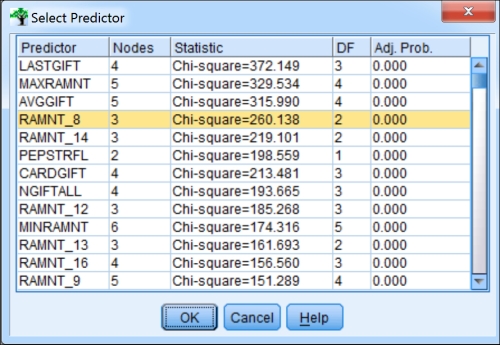
The figure shows
RAMNT_8, but your results may differ somewhat as CHAIDtakes an internal partition and therefore does not use all of the data. The slight differences can change the ranking of similar variables. Allow the branch to grow on your selected variable.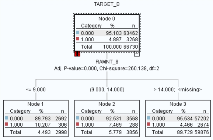
Now we will break away the missing data into its own category. Repeat the steps leading up to this branch, but before clicking on the Grow button, select Custom and at the bottom, set Missing values into as Separate Node.

Sometimes SMEs will have a particular interest in a variable because it has been known to be valuable in the past, or they are invested in the variable in some way. Even though it is well down the list, choose the variable
Wealth2and force it to branch while ensuring that missing values are placed into a Separate node.
There are several advantages to exploring data in this way with CHAID. If you have accidentally included perfect predictors it will become obvious in a hurry. This recipe is dedicated to this phenomenon. Another advantage is that most SMEs find CHAID rather intuitive. It is easy to see what the relationships are without extensive exposure to the technique. Meanwhile, as an added benefit, the SMEs are becoming acquainted with a technique that might also be used during the modeling phase. As we have seen, CHAID can show missing data as a Separate node. This feature is shown to be useful in the Binning scale variables to address missing data recipe in Chapter 3, Data Preparation – Clean. By staying in interactive mode, the trees are kept simple; also, we can force any variable to branch even if it is not near the top of the list. Often SMEs can be quite adamant that a variable is important, while the data shows them otherwise. There are countless reasons why this might be the case, and the conversation should be allowed to unfold. One is likely to learn a great deal trying to figure out why a variable that seemed promising is not performing well in the CHAID model.
Let's examine the CHAID tree a bit more closely. The root node shows the total sample size and the percentage in each of the two categories. In the figures in this recipe, the red group is the donors group. Notice that the more recent their LASTGIFT was, the more likely that they donated. Starting with 8.286 percent for the less than or equal to 9 group, dropping down to 3.476 percent for the less than 19 group. Note that when you add up the child nodes, you get the same number as the number in the root node.
It is recommended that you take a screenshot of at least the top 10 or so variables of interest to management or SMEs. It is a good precaution to place the images on slides, since you will be able to review and discuss without waiting for Modeler to process. Having said that, it is an excellent idea to be ready to further explore the data using this technique on live data during the meeting.
Cleaning data includes detecting and eliminating outliers. When outliers are viewed as a property of individual variables, it is easy to examine a data set, one variable at a time, and identify which records fall outside the usual range for a given variable. However, from a multivariate point of view, the concept of an outlier is less obvious; individual values may fall within accepted bounds but a combination of values may still be unusual.
The concept of multivariate outliers is used a great deal in anomaly detection, and this can be used both for data cleaning and more directly for applications such as fraud detection. Clustering techniques are often used for this purpose; in effect a clustering model defines different kinds of normal (the different clusters) and items falling outside these definitions may be considered anomalous. Techniques of anomaly detection using clustering vary from sophisticated, perhaps using multiple clustering models and comparing the results, through single-model examples such as the use of TwoStep in Modeler's Anomaly algorithm, to the very simple.
The simplest kind of anomaly detection with clustering is to create a cluster model with only one cluster. The distance of a record from the cluster center can then be treated as a measure of anomaly, unusualness or outlierhood. This recipe shows how to use a single-cluster K-means model in this way, and how to analyze the reasons why certain records are outliers.
This recipe uses the following files:
Data file:
cup98LRN.txtStream file:
Single_Cluster_Kmeans.strClementine output file:
Histogram.cou
To use a single cluster K-means as an alternative to anomaly detection:
Open the stream
Single_Cluster_Kmeans.strby clicking on File | Open Stream.Edit the Type node near the top-left of the stream; note that the customer ID and zip code have been excluded from the model, and the other 5 fields have been included as inputs.
Run the Histogram node
$KMD-K-Meansto show the distribution of distances from the cluster center. Note that a few records are grouped towards the upper end of the range.Open the output file
Histogram.couby selecting the Outputs tab at the top-right of the user interface, right-click in this pane to see the pop-up menu, select Open Output from this menu, then browse and select the fileHistogram.cou. You will see the graph in the following figure, including a boundary (the red line) that was placed manually to identify the area of the graph that, visually, appears to contain outliers. The band to the right of this line was used to generate the Select node and Derive node included in the stream, both labeledband2.
Run the Table node outliers; this displays the 8 records we have identified as outliers from the histogram, including their distance from the cluster center, as shown in the following screenshot. Note that they are all from the same cluster because there is only one cluster.

So far we have used the single-cluster K-means model to identify outliers, but why are they outliers? We can create a profile of these outliers to explain why they are outliers, by creating a rule-set model using the C5.0 algorithm to distinguish items that are in band2 from those that are not. This is a common technique used in Modeler to find explanations for the behavior of clustering models that are difficult to interrogate directly. The following steps show how:
Edit the Type node near the lower-right of the stream, as shown in the following screenshot. This is used to create the C5.0 rule-set model; note that the inputs are the same as for the initial cluster model, both outputs of the cluster model have been excluded, and the target is the derived field
band2, a Boolean that identifies the outliers.
Browse the C5.0 model,
band2and then use the Model pane to see all the rules and their statistics, as shown in the following screenshot. All the rules are highly accurate; even though they are not perfect, this is a successful profiling model in that it can distinguish reliably between outliers and others. This model shows how the cluster model has defined outliers: those records that have the rare valuesUandJfor theGENDERfield. The even more rare valueChas not been identified, because its single occurrence was insufficient to have an impact on the model.
Imagine a five-dimensional scatter-plot showing the 5 variables used for the cluster model and normalized. The records from the data set appear as a clump, and somewhere within that clump is its center of gravity. Some items fall at the edges of this clump; some may be visually outside it. The clump is the cluster discovered by K-means, and the items falling visually outside the clump are outliers.
Assuming the clump to be roughly spherical, the items outside the clump will be those at the greatest distance from its center, and have a gap between them and the edges of the clump. This corresponds to the gap in the histogram where we create a band of outliers from the histogram, which we have used manually to identify the band of outliers. The C5.0 rule-set is a convenient way to see a description of these outliers, more specifically how they differ from items inside the clump.
The final step mentions that the unique value C in the GENDER field has not been discovered in this instance because it is too rare to have an impact on the model. In fact, it is only too rare to have an impact on the relatively simplistic single-cluster model. It is possible for a K-means model to discover this outlier, and it will do so if used with its default setting of 5 clusters. This illustrates that the technique of using the distance from the cluster center to find outliers is more general than the single-cluster technique and can be used with any K-means model, or any clustering model that can output this distance.
With great regularity the mere presence or absence of data in the input variable tells you a great deal. Dates are a classic example. Suppose LastDateRented_HorrorCategory is NULL. Does that mean that the value is unknown? Perhaps we should replace it with the average date of the horror movie renters? Please don't! Obviously, if the data is complete, the failure to find Jane Renter in the horror movie rental transactions much more likely means that she did not rent a horror movie. This is such a classic scenario you will want a series of simple tricks to deal with this type of missing data efficiently so that when the situation calls for it you can easily create NULL flag variables for dozens (or even all) of your variables.
To use an @NULL multiple Derive node to explore missing data, perform the following steps:
Run the Data Audit and examine the resulting Quality tab. Note that a number of variables are complete but many have more than 5 percent NULL. The Filter node on the stream allows only the variables with a substantial number of NULL values to flow downstream.
Add a Derive node, and edit it, by selecting the Multiple option. Include all of the scale variables that are downstream of the Filter node. Use the suffix
_null, and select Flag from the Derive as drop-down menu.
Add another Filter node and set it to allow only the new variables plus TARGET_B to flow downstream.
Add a Type node forcing TARGET_B to be the target. Ensure that it is a flag measurement type.
Add a Data Audit node. Note that some of the new NULL flag variables may be related to the target, but it is not easy to see which variables are the most related.
Add a Feature Selection Modeling node and run it. Edit the resulting generated model. Note that a number of variables are predictive of the target.

There is no substitute for lots of hard work during Data Understanding. Some of the patterns here could be capitalized upon, and others could indicate the need for data cleaning. The Using the Feature Selection node creatively to remove or decapitate perfect predictors recipe in Chapter 2, Data Preparation – Select, shows how circular logic can creep into our analysis.
Note the large number of data and amount-related variables in the Generated model. These variables indicate that the potential donor did not give in those time periods. Failing to give in one time period is predicted with failing to give in another; it makes sense. Is this the best way to get at this? Perhaps a simple count would do the trick, or perhaps the number of recent donations versus total donations.

Also note the TIMELAG_null variable. It is the distance between the first and second donation. What would be a common reason that it would be NULL? Obviously the lack of a second donation could cause that problem. Perhaps analyzing new donors and established donors separately could be a good way of tackling this. The Using a full data model/partial data model approach to address missing data recipe in Chapter 3, Data Preparation – Clean, is built around this very idea. Note that neither imputing with the mean, nor filling with zero would be a good idea at all. We have no reason to think that one time and two time donors are similar. We also know for a fact that the time distance is never zero.
Note the Wealth2_null variable. What might cause this variable to be missing, and for the missing status alone to be predictive? Perhaps we need a new donor to be on the mailing list for a substantial time before our list vendor can provide us that information. This too might be tackled with a new donor/established donor approach.
The Using the Feature Selection node creatively to remove or decapitate perfect predictors recipe in Chapter 2, Data Preparation – Select
The Using CHAID stumps when interviewing an SME recipe in this chapter
The Binning scale variables to address missing data recipe in Chapter 3, Data Preparation – Clean
The Using a full data model/partial data model approach to address missing data recipe in Chapter 3, Data Preparation – Clean
It is quite common that the data miner has to rely on others to either provide data or interpret data, or both. Even when the data miner is working with data from their own organization there will be input variables that they don't have direct access to, or that are outside their day-to-day experience.
Are zero values normal? What about negative values? Null values? Are 1500 balance inquiries in a month even possible? How could a wallet cost $19,500? The concept of outliers is something that all analysts are familiar with. Even novice users of Modeler could easily find a dozen ways of identifying some. This recipe is about identifying outliers systematically and quickly so that you can produce a report designed to inspire curiosity.
There is no presumption that the data is in error, or that they should be removed. It is simply an attempt to put the information in the hands of Subject Matter Experts, so quirky values can be discussed in the earliest phases of the projects. It is important to provide whichever primary keys are necessary for the SMEs to look up the records. On one of the author's recent projects, the team started calling these reports quirk reports.
We will start with the Outlier Report.str stream that uses the TELE_CHURN_preprep data set.
Open the stream
Outlier Report.str.
Add a Data Audit node and examine the results.

Adjust the stream options to allow for 25 rows to be shown in a data preview. We will be using the preview feature later in the recipe.

Add a Statistics node. Choose Mean, Min, Max, and Median for the variables
DATA_gb,PEAK_mins, andTEXT_count. These three have either unusually high maximums or surprising negative values as shown in the Data Audit node.Consider taking a screenshot of the Statistics node for later use.

Add a Sort node. Starting with the first variable,
DATA_gb, sort in ascending order.
Add a Filter node downstream of the Sort node dropping
CHURN,DROPPED_CALLS, andLATE_PAYMENTS. It is important to work with your SME to know which variables put quirky values into context.
Preview the Filter node. Consider the following screenshot:

Reverse the sort, now choosing descending order, and preview the Filter node. Consider the following screenshot for later use:

Sort in descending order on the next variable,
PEAK_mins. Preview the Filter node.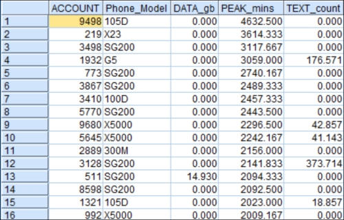
Finally sort the variable,
TEXT_count, in descending order and preview the Filter node.
Examine
Outliers.docxto see an example of what this might look like in Word.
There is no deep theoretical foundation to this recipe; it is as straightforward as it seems. It is simply a way of quickly getting information to an SME. They will not be frequent Modeler users. Also summary statistics only give them a part of the story. Providing the min, max, mean and median alone will not allow an SME to give you the information that you need. If there is a usual min such as a negative value, you need to know how many negatives there are, and need at least a handful of actual examples with IDs. An SME might look up to values in their own resources and the net result could be the addition of more variables to the analysis. Alternatively, negative values might be turned into nulls or zeros. Negative values might be deemed out of scope and removed from the analysis. There is no way to know until you assess why they are negative. Sometimes values that are exactly zero are of interest. High values, NULL values, and rare categories are all of potential interest. The most important thing is to be curious (and pleasantly persistent) and to inspire collaborators to be curious as well.
Model instability would typically be described as an issue most noticeably during the evaluation phase. Model instability usually manifests itself as a substantially stronger performance on the Train data set than on the Test data set. This bodes ill for the performance of the model on new data; in other words, it bodes ill for the practical application of the model to any business problem. Veteran data miners see this coming well before the evaluation phase, however, or at least they hope they do. The trick is to spot one of the most common causes; model instability is much more likely to occur when the same inputs are competing for the same variance in the model. In other words, when the inputs are correlated with each other to a large degree, it can cause problems. The data miner can also get themselves into hot water with their own behavior or imprudence. Overfitting, discussed in the Introduction of Chapter 7, Modeling – Assessment, Evaluation, Deployment, and Monitoring, can also cause model instability. The trick is to spot potential problems early. If the issue is in the set of inputs, this recipe can help to identify which inputs are at issue. The correlation matrix recipe and other data reduction recipes can assist in corrective action.
This recipe also serves as a cautionary tale about giving the Feature Selection node a heavier burden than it is capable of carrying. This node looks at the bivariate relationships of inputs with the target. Bivariate simply means two variables and it means that Feature Selection is blind to what might happen when lots of inputs attempt to collaborate together to predict the target. Bivariate analyses are not without value, they are critical to the Data Understanding phase, but the goal of the data miner is to recruit a team of variables. The team's performance is based upon a number of factors, only one of which is the ability of each input to predict the target variable.
To detect potential model instability using the Partition and Feature Selection nodes, perform the following steps:
Open the stream,
Stability.str.
Edit the Partition node, click on the Generate seed button, and run it. (Since you will not get the same seed as the figure shown, your results will differ. This is not a concern. In fact, it helps illustrate the point behind the recipe.)

Run the Feature Selection Modeling node and then edit the resulting generated model. Note the ranking of potential inputs may differ if the seed is different.

Edit the Partition node, generate a new seed, and then run the Feature Selection again.
Edit the Feature Selection generated model.

For a third and final time, edit the Partition node, generate a new seed, and then run the Feature Selection. Edit the generated model.

At first glance, one might anticipate no major problems ahead. RFA_6, which is the donor status calculated six campaigns ago, is in first place twice and is in third place once. Clearly it provides some value, so what is the danger in proceeding to the next phase? The change in ranking from seed to seed is revealing something important about this set of variables. These variables are behaving like variables that are similar to each other. They are all descriptions of past donation behavior at different times. The larger the number after the underscore, the further back in time they represent. Why isn't the most recent variable, RFA_2, shown as the most predictive? Frankly, there is a good chance that it is the most predictive, but these variables are fighting over top status in the small decimal places of this analysis. We can trust Feature Selection to alert us that they are potentially important, but it is dangerous to trust the ranking under these circumstances, and it certainly doesn't mean than if we were to restrict our inputs to the top ten that we would get a good model.
The behavior revealed here is not a good indication of how these variables will behave in a model, a classification tree, or any other multiple input techniques. In a tree, once a branch is formed using RFA_6, the tendency would be for the model to seek a variable that sheds light on some other aspect of the data. The variable used to form the second branch would likely not be the second variable on the list because the first and second variables are similar to each other. The implication of this is that, if RFA_4 were chosen as the first branch, RFA_6 might not be chosen at all.
Each situation is different, but perhaps the best option here is to identify what these related variables have in common and distill it into a smaller set of variables. To the extent that these variables have a unique contribution to make—perhaps in the magnitude of their distance in the past—that too could be brought into higher relief during data preparation.