


Loading, Tidying, and Cleaning Data in the tidyverse
Cleaning data is a crucial step in the data science process. It involves identifying and correcting errors, inconsistencies, and missing values in the data, as well as formatting and structuring the data in a way that makes it easy to work with. This allows the data to be used effectively for analysis, modeling, and visualization. The R tidyverse is a collection of packages designed for data science and includes tools for data manipulation, visualization, and modeling. The dplyr and tidyr packages are two of the most widely used packages within the tidyverse for data cleaning. dplyr provides a set of functions for efficiently manipulating large datasets, such as filtering, grouping, and summarizing data. tidyr is specifically designed for tidying (or restructuring) data, making it easier to work with. It provides functions for reshaping data, such as gathering and spreading columns, and allows for the creation of a consistent structure in the data. This makes it easier to perform data analysis and visualization. Together, these packages provide powerful tools for cleaning and manipulating data in R, making it a popular choice among data scientists. In this chapter, we will look at tools and techniques for preparing data in the tidyverse set of packages. You will learn how to deal with different formats and quickly interconvert them, merge different datasets, and summarize them. You will also learn how to bring data from outside sources not in handy files into your work.
In this chapter, we will cover the following recipes:
- Loading data from files with
readr - Tidying a wide format table into a tidy table with
tidyr - Tidying a long format table into a tidy table with
tidyr - Combining tables using join functions
- Reformatting and extracting existing data into new columns using
stringr - Computing new data columns from existing ones and applying arbitrary functions using
mutate() - Using
dplyrto summarize data in large tables - Using
datapastato create R objects from cut-and-paste data
Technical requirements
We will use renv to manage packages in a project-specific way. To use renv to install packages, you will first need to install the renv package. You can do this by running the following commands in your R console:
- Install
renv:install.packages("renv") - Create a new
renvenvironment:renv::init()
This will create a new directory called .renv in your current project directory.
- You can then install packages with the following command:
renv::install_packages()
- You can also use the
renvpackage manager to installBioconductorpackages by running the following command:renv::install("bioc::package name") - For example, to install the
Biobasepackage, you would run the following command:renv::install("bioc::Biobase") - You can use
renvto install development packages from GitHub like this:renv::install("user name/repo name") - For example, to install the
danmacleanuserrbioinfcookbookpackage, you would run the following command:renv::install("danmaclean/rbioinfcookbook")
You can also install multiple packages at once by separating the package names with a comma. renv will automatically handle installing any required dependencies for the packages you install.
Under renv, all packages will be installed into the local project directory and not the main central library, meaning you can have multiple versions of the same package—a specific one for each project.
All the sample data you need for this package is in the specially created danmaclean/rbioinfcookbook data package on GitHub. The data will become available in your project after installing that.
For this chapter, we’ll need the following packages:
- Regular packages:
dplyrfsreadrtidyrstringrpurrr
- GitHub:
danmaclean/rbioinfcookbook
- Custom install:
datapasta
In addition to these packages, we will also need some R tools such as conda; all these will be described when needed.
Further information
The packages that require a custom install procedure will be described in the relevant recipes.
In R, it is normal practice to load a library and use functions directly by name. Although this is great in short interactive sessions, it can cause confusion when many packages are loaded at once and share function names. To clarify which package and function I am using at a given moment, I will occasionally use the packageName::functionName() convention.
Sometimes, in the middle of a recipe I’ll interrupt the code to dive into some intermediate output or to look at the structure of an object. When that happens, you’ll see a code block where each line begins with ## (double hash symbols). Consider the following command:
letters[1:5]
This will give us the following output:
## a b c d e
Note that the output lines are prefixed with ##.
Loading data from files with readr
The readr R package is a package that provides functions for reading and writing tabular data in a variety of formats, including comma-separated values (CSV), tab-separated values (TSV), and delimiter-separated files. It is designed to be flexible and stop helpfully when data changes or unexpected items appear in the input. The two main advantages over base R functions include consistency in interface and output and the ability to be explicit about types and inspect those types.
This latter advantage can help to avoid errors when reading data, as well as make data cleaning and manipulation easier. readr functions can also automatically infer the data types of each column, which can be useful for a preliminary inspection of large datasets or when the data types are not known.
Consistency in interface and output is one of the main advantages of readr functions. readr functions provide a consistent interface for reading different types of data, which can make it easier to work with multiple types of files. For example, the read_csv() function can be used to read CSV files, while the read_tsv() function can be used to read TSV files. Additionally, readr functions return a tibble, a modern version of a data frame that is more consistent in its output and easier to read than the base R data frame.
Getting ready
For this recipe, we’ll need the readr and rbioinfcookbook packages. The latter contains a census_2021.csv file that carries UK census data from 2021, from the UK Office for National Statistics (https://www.ons.gov.uk/). You will need to inspect it, especially its header, to understand the process in this recipe. The first step shows you how to find where the file is on your filesystem.
Note the delimiters in the file are commas (,) and that the first seven lines contain metadata that isn’t part of the main data. Also, look at the messy column headings and note that the numbers themselves are internally delimited by commas.
How to do it…
We begin by getting a filename for the sample in the package:
- Load the package and get a filename:
library(readr)filename <- fs::path_package("extdata", "census_2021.csv", package="rbioinfcookbook" ) - Specify a vector of new names for columns:
col_names = c( c("area_code", "country", "region", "area_name", "all_persons", "under_4"), paste0(seq(5, 85, by = 5),"_to_",seq(9, 89, by =5)),c("over_90")) - Set the column types based on new names and contents:
col_types = cols( area_code = col_character(), country = col_factor(levels = c("England", "Wales")), region = col_factor(levels = c("North East", "Yorkshire Humber", "East Midlands", "West Midlands", "East of England", "London", "South East", "South West", "Wales"), ordered = TRUE ), area_name = col_character(), .default = col_number()) - Put it together and read the file:
df <- read_csv(filename, skip = 8, col_names = col_names, col_types = col_types )
And with that, we’ve loaded in a file with careful checking of the data types.
How it works…
Step 1 loads the library(readr) package. This package contains functions for reading and writing tabular data in a variety of formats, including CSV. The fs::path_package("extdata", "census_2021.csv", package="rbioinfcookbook") function is used to create a file path to the census_2021.csv file. It simply finds the place where the rbioinfcookbook package was installed and looks inside the extdata directory for the file, then it returns the full file path that leads to the file. Quite often, we would see the system.file() function used for this purpose. system.file() is a fine choice when everything works, but when it can’t find the file, it returns a blank string, which can be hard to debug. fs::path_package() is nicer to work with and will return an error when it can’t find the file.
In step 2, a vector of new column names is specified by the code. The vector contains several strings for the first few column names, and then a sequence of strings is created and a long list of age-related columns is created by concatenating two sequences of numbers. The resulting vector is stored in the col_names variable.
In step 3, we specify the R type we want each column to be. The categorical columns are set explicitly to factors, with the region being ordered explicitly in a rough geographical northeast to southwest way. The area_name column contains over 300 names, so we won’t make them an explicit factor and stick with it as a general text containing character type. The rest of the columns contain numeric data, so we make that the default with .default.
Finally, the read_csv() function is used to read the file specified in step 1 and create a data frame. The skip argument is used to skip the first eight rows, which include the metadata in the file and the messy header, the col_names argument is used to specify the new column names stored in col_names, and the col_types argument is used to specify the column types stored in col_types.
There’s more…
We used the read_csv() function for comma-separated data, but many more functions are available for different delimiters:
|
Function |
Delimiter |
|
|
CSV |
|
|
TSV |
|
|
User-specified delimited files |
|
|
Fixed-width files |
|
|
Whitespace-separated files |
|
|
Web log files |
Table 2.1 – Parser functions and the type of input file delimiter they work on in readr
For different local conventions on—for example—decimal separators and grouping marks, you can use the locale functions.
See also
The data.table package has a similar aim to readr and is especially good for very large data frames where compute speed is important.
Tidying a wide format table into a tidy table with tidyr
The tidyr package in R is a package that provides tools for tidying and reshaping data. It is designed to make it easy to work with data in a consistent and structured format, which is known as a tidy format. Tidy data is a standard way of organizing data that makes it easy to perform data analysis and visualization.
The main principles of tidy data are as follows:
- Each variable forms a column
- Each observation forms a row
- Each type of observational unit forms a table
Data in a tidy format is easier to work with because the structure of the data is consistent, facilitating operations such as filtering, grouping, and reshaping the data. Tidy data is also more compatible with various data visualization and analysis tools, such as ggplot2, dplyr, and other tidyverse packages.
Our aim in this recipe will be to take a wide format data frame where a lot of information is hiding in column names and squeeze and reformat them into a data column of their own and rationalize them in the process.
Getting ready
We’ll need the rbioinfcookbook and tidyr packages. We’ll use the finished output from recipe 1, which is saved in the package.
How to do it…
We have to use just one function, but the options are many.
Specify the transformation to the table:
library(rbioinfcookbook)library(dplyr)
library(tidyr)
long_df <- census_df |>
  rename("0_to_4" = "under_4", "90_to_120" = "over_90") |>
  pivot_longer(
    cols = contains("_to_"),
    names_to = c("age_from", "age_to"),
    names_pattern = "(.*)_to_(.*)",
    names_transform = list("age_from" = as.integer,
                         age.to = as.integer),
    values_to = "count"
  )
And that’s it. This short recipe is very dense, though.
How it works…
The tidyr package has functions that work by allowing the user to specify a particular transformation that will be applied to the data frame to generate a new one. In this single step, we specify a table row-count increasing operation that will find all the columns that contain age information. Next, we split the title of that column into data for two new columns—one for the lower boundary of the age category and one for the upper boundary of the age category. Then, we change the type of those new columns to integer and, lastly, put the actual counts in a new column.
The first function in this pipeline is code from dplyr, which helps us rename column headings. Our age data column names are largely consistent, except for the lower bound and the upper one, so we rename those columns to match the pattern of the others, simplifying the transform specification.
The pivot_longer() function specifies the transform in the arguments, with the cols argument we choose to operate on any columns containing the text to. The names_pattern argument takes a regular expression (regex) that captures the bits of text before and after the to string in the column names and uses them as values for the columns defined in the names_to argument. The actual counts from the cell are put into a new column called counts. The transformation is then applied in one step and reduces the data frames column count to eight, increasing the row count to 6,935, and in the process making the data tidy and easier to use in downstream packages.
See also
The recipe uses a regex to describe a pattern in text. If you haven’t seen these before and need a primer, try typing ?"regular expression" to view the R help on the topic.
Tidying a long format table into a tidy table with tidyr
In this recipe, we look at the complementary operation to that of the Tidying a wide format table into a tidy table with tidyr recipe. We’ll take a long table and split one of its columns out to make multiple new columns. Initially, this might seem like we’re now violating our tidy data frame requirement, but we do occasionally come across data frames that have more than one variable squeezed into a single column. As in the previous recipe, tidyr has a specification-based function to allow us to correct our data frame.
Getting ready
We’ll use the tidyr package and the treatment data frame in the rbioinfcookbook package. This data frame has four columns, one of which—measurement—has got two variable names in it that need splitting into columns of their own.
How to do it…
In stark contrast to the Tidying a wide format table into a tidy table with tidyr recipe, this expression is extremely terse; we can tidy the wide table very easily:
library(rbioinfcookbook)library(tidyr)
treatments |>
  pivot_wider(
    names_from = measurement,
    values_from = value
  )
This is so simple because all the data we need is already in the data frame.
How it works…
In this very simple-looking recipe, the specification is gloriously clear: simply take the measurement column and create new column names from its values, moving the value appropriately. The names_from argument specifies the column to split, and values_from specifies where its values come from.
There’s more…
It is quite possible to incorporate values from more than one column at a time; just pass a vector of columns to the names_from argument, and you can format the computed column names in the output with names_glue.
Combining tables using join functions
Joining rectangular tables in data science is a powerful way to combine data from multiple sources, allowing for more complex and detailed analysis. The process of joining tables involves matching rows from one table with corresponding rows in another table, based on shared columns or keys. The ability to join tables allows data scientists to gather information from different sources and can also be used to clean and prepare data for analysis by eliminating duplicates or filling in missing values. Note that although the joining process is powerful and useful, it isn’t magic and is actually a common source of errors. The user must take care that the operation was successful in the way that they intended and that combining data doesn’t create unexpected combinations, especially empty cells and repeated rows.
The dplyr package provides functions for manipulating and cleaning data, including a function called join() that can be used to join tables based on one or more common columns. The join() function supports several types of joins, including inner, left, right, and full outer joins. In this recipe, we’ll look at how each of these joins works.
Getting ready
We’ll need the dplyr package and the rbioinfcookbook package, which will give us a short gene expression dataset of just 10 Magnaporthe oryzae genes, and related annotation data of approximately 60,000 rows for the entire genome.
How to do it…
The process will begin with loading a data frame from the data package. The mo_gene_exp, mo_go_acc, and mo_go_evidence objects are all available as data objects when you load the rbioinfcookbook library, so we don’t have to try to load them from the file. You will have seen this behavior in numerous R tutorials before. For our work, this mimics the situation where you will already have gone through the process of loading in the data from a file on disk or received a data frame from an upstream function.
The following will help us to join tables together:
- Load the data and add terms to genes:
library(rbioinfcookbook)library(dplyr)x <- left_join(mo_gene_exp, mo_terms, by = c('gene_id' = 'Gene stable ID')) - Add accession numbers:
y <- right_join(mo_go_acc, x, by = c( 'Gene stable ID' = 'gene_id' ) )
- Add evidence code:
z <- inner_join(y, mo_go_evidence, by = c('GO term accession' = 'GO term evidence code')) - Compare the direction of joins:
a <- right_join(x, mo_go_acc, by = c( 'gene_id' = 'Gene stable ID') )
- Stack two data frames:
mol_func <- filter(mo_go_evidence, `GO domain` == 'molecular_function')cell_comp <- filter(mo_go_evidence, `GO domain` == 'cellular_component')bind_rows(mol_func, cell_comp)
- Put two data frames side by side:
small_mol_func <- head(mol_func, 15)small_cell_comp <- head(cell_comp, 15)bind_cols(small_mol_func, small_cell_comp)
And with that, we have joined data frames into one in most ways possible.
How it works…
The code joins different data frames in various ways. The mo_gene_exp, mo_terms, mo_go_acc, and mo_go_evidence objects are data frames, and they are loaded using the rbioinfcookbook library. Then, the first operation is to add terms to genes using the left_join() function. The left_join() function joins the mo_gene_exp and mo_terms data frames on the gene_id column of the mo_gene_exp data frame and the Gene stable ID column of the mo_terms data frame. Note the increase in rows as well as columns because of the multiple matching rows.
By step 2, we’re adding accession numbers using the right_join() function to join the mo_go_acc data frame and the result of the first join (x) on the Gene stable ID column of the mo_go_acc data frame and the gene_id column of the x data frame. Ordering the data frames this way minimizes the number of rows; see step 5 for how the converse goes. Note that the right_join() function returns the full set of rows from the right data frame.
Step 3’s inner_join() function demonstrates that only the rows shared are returned. The remaining steps create subsets of the mo_go_evidence data frame based on the component to highlight how bind_rows() does a name-unaware stacking and bind_cols() does a blind left-right paste/concatenation of data frames. These last two functions are quick and easy but do not do anything clever, so be sure that the data can be properly joined this way.
Reformatting and extracting existing data into new columns using stringr
Text manipulation is important in bioinformatics as it allows, among other things, for efficient processing and analysis of DNA and protein sequence annotation data. The R stringr package is a good choice for text manipulation because it provides a simple and consistent interface for common string operations, such as pattern matching and string replacement. stringr is built on top of the powerful stringi manipulation library, making it a fast and efficient tool for working with arbitrary strings. In this recipe, we’ll look at rationalizing data held in messy FAST-All (FASTA)-style sequence headers.
Getting ready
We’ll use the Arabidopsis gene names in the ath_seq_names vector provided by the rbioinfcookbook package and the stringr package.
How to do it…
To reformat gene names using stringr, we can proceed as follows:
- Capture the
ATxGxxxxxformat IDs:library(rbioinfcookbook)library(stringr)ids <- str_extract(ath_seq_names, "^AT\\dG.*\\.\\d")
- Separate the string into elements and extract the description:
description <- str_split(ath_seq_names, "\\|", simplify = TRUE)[,3] |> str_trim()
- Separate the string into elements and extract the gene information:
info <- str_split(ath_seq_names, "\\|", simplify = TRUE)[,4] |> str_trim()
- Match and recall the chromosome and coordinates:
chr <- str_match(info, "chr(\\d):(\\d+)-(\\d+)")
- Find the number of characters the strand information begins at and use that as an index:
strand_pos <- str_locate(info, "[FORWARD|REVERSE]")strand <- str_sub(info, start=strand_pos, end=strand_pos+1)
- Extract the length information:
lengths <- str_match(info, "LENGTH=(\\d+)$")[,2]
- Combine all captured information into a data frame:
results <- data.frame( ids = ids, description = description, chromosome = as.integer(chr[,2]), start = as.integer(chr[,3]), end = as.integer(chr[,4]), strand = strand, length = as.integer(lengths))
And that gives us a very nice, reformatted data frame.
How it works…
The R code uses the stringr library to extract, split, and manipulate information from a vector of sequence names (ath_seq_names) and assigns the resulting information to different variables. The rbioinfcookbook library provides the initial ath_seq_names vector.
The first step of the recipe uses the str_extract() function from stringr to extract a specific pattern of characters. The "^AT\dG.*.\d" regex matches any string that starts with "AT", followed by one digit, then "G", then any number of characters, then a dot, and finally one digit. stringr operations are vectorized so that all entries in them are processed.
Steps 2 and 3 are similar and use the str_split() function to split the seq_names vector by the "|" character; the simplify option returns a matrix of results with a column for each substring. The str_trim() function removes troublesome leading and trailing whitespace from the resulting substring. The third and fourth columns of the resulting matrix are saved.
The following line of code uses the str_match() function to extract specific substrings from the info variable that match the "chr(\d):(\d+)-(\d+)" regex. This regex matches any string that starts with "chr", followed by one digit, then ":", then one or more digits, then "-", and finally one or more digits. The '()' bracket symbols mark the piece of text to save; each saved piece goes into a column in the matrix.
The next line of code uses the str_locate() function to find the position of the first occurrence of either FORWARD or REVERSE in the info variable. The resulting position is then used to extract the character at that position using str_sub(). The last line of code uses the str_match() function to extract the substring that starts with "LENGTH=" and ends with one or more digits from the info variable.
Finally, the code creates a data frame result by combining the extracted and subsetted variables, assigning appropriate types for each column.
Computing new data columns from existing ones and applying arbitrary functions using mutate()
Data frames are the core data structure in R for storing and manipulating tabular data. They are similar to a table in a relational database or a spreadsheet, with rows representing observations and columns representing variables. The mutate() function in dplyr is used to add new columns to a data frame by applying a function or calculation to existing columns; it can be used on both data frames and nested datasets. A nested dataset is a data structure that contains multiple levels of information, such as lists or data frames within data frames.
Getting ready
In this recipe, we’ll use a very small data frame that will be created in the recipe and the dplyr, tidyr, and purrr packages.
How to do it…
The functionality offered by the mutate() pattern is exemplified in the following steps:
- Add some new columns:
library(dplyr)df <- data.frame(gene_id = c("gene1", "gene2", "gene3"), tissue1 = c(5.1, 7.3, 8.2), tissue2 = c(4.8, 6.1, 9.5))df <- df |> mutate(log2_tissue1 = log2(tissue1), log2_tissue2 = log2(tissue2)) - Conditionally operate on columns:
df |> mutate_if(is.numeric, log2)df |> mutate_at(vars(starts_with("tissue")), log2) - Operate across columns:
library(dplyr)df <- data.frame(gene_id = c("gene1", "gene2", "gene3"), tissue1 = c(5.1, 7.3, 8.2), tissue2 = c(4.8, 6.1, 9.5), tissue3 = c(8.5, 12.5, 6.5))df <- df |> rowwise() |> mutate(mean = mean(c(tissue1, tissue2, tissue3)), stddev = sd(c(tissue1, tissue2, tissue3)) ) - Operate on nested data:
df <- data.frame(gene_id = c("gene1", "gene2", "gene3"), tissue1_value = c(5.1, 7.3, 8.2), tissue1_pvalue = c(0.01, 0.05, 0.001), tissue2_value = c(4.8, 6.1, 9.5), tissue2_pvalue = c(0.03, 0.04, 0.001) ) |> tidyr::nest(-gene_id, .key = "tissue")df <- df |> mutate(tissue = purrr::map(tissue, ~ mutate(.x, value_log2 = log2(.[1]),pvalue_log2 = log2(.[2])) ))
These are the various ways we can work with mutate() on different data frames to different ends.
How it works…
In step 1, we start by creating a data frame containing three genes, with columns representing the values of each gene. Then, we use the [mutate(){custom-style='P - Code'} function in its most basic form to apply the log2 transformation of the values into new columns.
In step 2, we apply the transformation conditionally with mutate_if(), which applies the specified function to all columns that match the specified condition (in this case, is.numeric), and mutate_at() to apply the log2 function to all columns that start with the name tissue.
In step 3, we create a bigger data frame of expression data and then use the rowwise() function in conjunction with mutate() to add two new columns, mean and stddev, which contain the mean and standard deviation of the expression values across all three tissues for each gene. If we just use mutate() on the vector, the function will be applied to the entire column instead of the rows. As we need to calculate the mean and standard deviation of the expression values across all tissues, this would be difficult to achieve just by using mutate() on vectors in the standard column-wise fashion.
Finally, we look at using mutate() in nested data frames. We begin by creating a data frame of genes and expression values and use the nest() function to create a nested data frame. We can then use the combination of mutate() and map() functions from the purrr package, to extract the tissue1_value and tissue2_value columns from the nested part of the data frame.
Using dplyr to summarize data in large tables
Split-apply-combine is a technique used in data science to analyze and manipulate large datasets by breaking them down into smaller, more manageable pieces, applying a function or operation to each piece, and then combining the results. It’s a powerful method for working with data because it allows you to process and analyze data in a way that is both efficient and interpretable. The process can be repeated multiple times to gain deeper insights into the data.
In the tidyverse, the dplyr package provides a set of tools for implementing the split-apply-combine technique; we’ll look at those in this recipe.
Getting ready
We will need the dplyr and tidyr packages for this recipe.
How to do it…
The functionality of the dplyr package for split-apply-combine techniques is shown in the following steps:
- Create the initial data frame:
chromosome_id <- c(1,1,1,2,2,3,3,3)gene_id <- c("A1","A2","A3","B1","B2","C1","C2","C3")strand <- c("forward","reverse","forward","forward", "reverse","forward","forward","reverse")length <- c(2000,1500,3000,2500,2000,1000,2000,3000)genes_df <- data.frame(chromosome_id,gene_id,strand,length) - Group on a single column:
library(dplyr)genes_df |> group_by(chromosome_id) |> summarise(total_length = sum(length))
- Group and summarize on multiple columns:
genes_df |> group_by(chromosome_id, strand) |> summarise( num_genes = n(), avg_length = mean(length) )
- Work on a nested data frame:
# Create a nested dataframechromosome_id <- c(1,1,1,2,2,3,3,3)gene_id <- c("A1","A2","A3","B1","B2","C1","C2","C3")strand <- c("forward","reverse","forward","forward","reverse","forward","forward","reverse")length <- c(2000,1500,3000,2500,2000,1000,2000,3000)genes_df <- data.frame(chromosome_id,gene_id,strand,length)genes_df$samples <- list(data.frame(sample_id=1:2, expression=c(2,3)), data.frame(sample_id=1:3, expression=c(3,4,5)), data.frame(sample_id=1:2, expression=c(4,5)), data.frame(sample_id=1:3, expression=c(5,6,7)), data.frame(sample_id=1:2, expression=c(6,7)), data.frame(sample_id=1:2, expression=c(1,2)), data.frame(sample_id=1:2, expression=c(2,3)), data.frame(sample_id=1:2, expression=c(3,4)) )genes_df |> tidyr::unnest() |> group_by(chromosome_id,strand) |> summarise(mean_expression = mean(expression))
These are a broad set of examples for the use of split-apply-combine in dplyr.
How it works…
Step 1 explicitly creates a data frame; we do it this way so that we can easily understand its structure.
In step 2, we use the method in its simplest form: the group_by() function is used to group the rows of a data frame based on the chromosome_id, and then we use summarise() to return a summary data frame. Step 3 is similar but shows how multiple grouping columns can be used to create more granular groups and how more than one summary function can be applied.
Step 4 is more complex; the new data frame is a nested data frame, and the samples list column contains a data frame of expression data in each cell. When using group_by() and summarise() functions on a nested data frame, you first need to access the nested data using the tidyr::unnest() function, then group and summarize as usual. Note that when using tidyr::unnest(), the new data frame will have multiple rows for each gene, one for each sample, so it’s important to group the data frame by the columns of interest.
Using datapasta to create R objects from cut-and-paste data
Being able to paste data into source code documents is useful for all sorts of reasons, not least because it allows for a reproducible example, also known as a reprex—a minimal, self-containedexample that demonstrates a problem or a concept. By including data in the source code, others can run the code and see the results for themselves, making it easier to understand and replicate the results.
The R datapasta package makes it easy to paste data into R source code documents. It provides a set of functions for converting data to and from R definitions and is extremely useful when creating static data objects in code examples, tests, or when sharing. In this recipe, you will learn how to use datapasta to bring external data into your source code documents by typing them in longhand.
Getting ready
We will use the datapasta package, though installing it is non-standard. Use this command:
renv::install("datapasta", repos = c(mm = "https://milesmcbain.r-universe.dev", getOption("repos"))) This should install the package using renv and make us ready to go. Remember to install renv the usual way if you don’t already have it.
How to do it…
The datapasta tool is implemented as an add-in for RStudio, so we begin by setting that up:
- Use the RStudio Tools | Addins | Browse Addins menu and then Keyboard Shortcuts. You get to choose which key combination you want to use for pasting.
- Click the middle column next to the operations, as shown in the following screenshot, and press the keys you want to use. The combination in Figure 2.1 is a good choice:
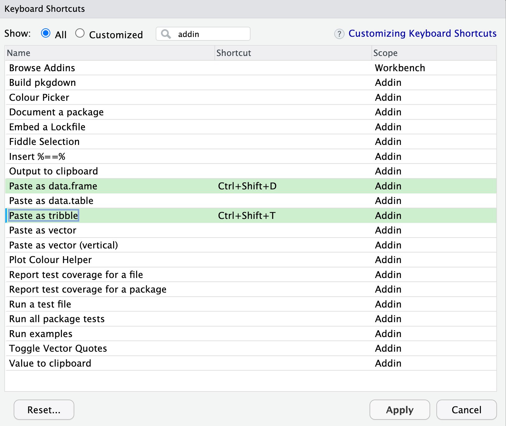
Figure 2.1 – Selecting key shortcuts
- Get a web table—for example, go to this page on Wikipedia: https://en.wikipedia.org/wiki/Tab-separated_values—and copy the whole text-based example table using the browser’s right-click Copy feature. This should put the text table in your copy/paste buffer. It should look like what’s shown in Figure 2.2:
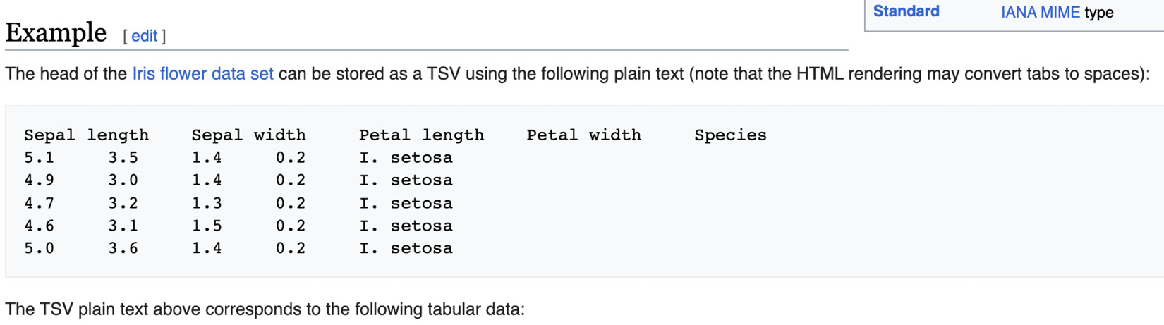
Figure 2.2 – Web data on Wikipedia
- Paste the table now in your copy/paste buffer into an R source document. Place the typing cursor at a suitable place in the source R document you’re working in and use the key combo to paste in the table.
So, with the preceding setup, we should be able to quickly take data from varied sources and coerce them into R objects for analysis.
How it works…
The datapasta package is really useful. The first step sets up our preferred paste keys for later use; the second step is simple, and we just go somewhere and find some data in the world we would like in our R source; and by the third step, we’re selecting the place to put the data definition and pasting it in. Our example goes from a table in a web page to this definition for an R object:
data.frame(  stringsAsFactors = FALSE,
      Sepal.length = c(5.1, 4.9, 4.7, 4.6, 5),
       Sepal.width = c(3.5, 3, 3.2, 3.1, 3.6),
      Petal.length = c(1.4, 1.4, 1.3, 1.5, 1.4),
       Petal.width = c(0.2, 0.2, 0.2, 0.2, 0.2),
           Species = c("I. setosa","I. setosa",
                       "I. setosa","I. setosa","I. setosa")
)
And that powerful little operation is how we can convert web data to source code very easily.
There’s more…
It’s possible to go the other way around, from some R object to a definition of that object using the dpasta() function, which can coerce data frames, tibbles, and vectors into definitions. This is really useful for reproducible examples. This example shows how to actually build the object with code so that we don’t have to share the file and everything is in one source document:
library(datapasta)mtcars |>
   dpasta()
This shows how the datapasta package is a super-useful tool for turning objects from the web and within R into code.