


 Download code from GitHub
TensorFlow is a popular library for implementing machine learning-based solutions. It includes a low-level API known as TensorFlow core and many high-level APIs, including two of the most popular ones, known as TensorFlow Estimators and Keras. In this chapter, we will learn about the basics of TensorFlow and build a machine learning model using logistic regression to classify handwritten digits as an example.
We will cover the following topics in this chapter:
- TensorFlow core:
- Tensors in TensorFlow core
- Constants
- Placeholders
- Operations
- Tensors from Python objects
- Variables
- Tensors from library functions
- Computation graphs:
- Lazy loading and execution order
- Graphs on multiple devices – CPU and GPGPU
- Working with multiple graphs
- Machine learning, classification, and logistic regression
- Logistic regression examples in TensorFlow
- Logistic regression examples in Keras
TensorFlow is a popular open source library that's used for implementing machine learning and deep learning. It was initially built at Google for internal consumption and was released publicly on November 9, 2015. Since then, TensorFlow has been extensively used to develop machine learning and deep learning models in several business domains.
To use TensorFlow in our projects, we need to learn how to program using the TensorFlow API. TensorFlow has multiple APIs that can be used to interact with the library. The TensorFlow APIs are divided into two levels:
- Low-level API: The API known as TensorFlow core provides fine-grained lower level functionality. Because of this, this low-level API offers complete control while being used on models. We will cover TensorFlow core in this chapter.
- High-level API: These APIs provide high-level functionalities that have been built on TensorFlow core and are comparatively easier to learn and implement. Some high-level APIs include Estimators, Keras, TFLearn, TFSlim, and Sonnet. We will also cover Keras in this chapter.
The TensorFlow core is the lower-level API on which the higher-level TensorFlow modules are built. In this section, we will go over a quick overview of TensorFlow core and learn about the basic elements of TensorFlow.
Tensors are the basic components in TensorFlow. A tensor is a multidimensional collection of data elements. It is generally identified by shape, type, and rank. Rank refers to the number of dimensions of a tensor, while shape refers to the size of each dimension. You may have seen several examples of tensors before, such as in a zero-dimensional collection (also known as a scalar), a one-dimensional collection (also known as a vector), and a two-dimensional collection (also known as a matrix).
A scalar value is a tensor of rank 0 and shape []. A vector, or a one-dimensional array, is a tensor of rank 1 and shape [number_of_columns] or [number_of_rows]. A matrix, or a two-dimensional array, is a tensor of rank 2 and shape [number_of_rows, number_of_columns]. A three-dimensional array is a tensor of rank 3. In the same way, an n-dimensional array is a tensor of rank n.
A tensor can store data of one type in all of its dimensions, and the data type of a tensor is the same as the data type of its elements.
Note
The data types that can be found in the TensorFlow library are described at the following link: https://www.tensorflow.org/api_docs/python/tf/DType.
The following are the most commonly used data types in TensorFlow:
TensorFlow Python API data type | Description |
| 16-bit floating point (half-precision) |
| 32-bit floating point (single-precision) |
| 64-bit floating point (double-precision) |
| 8-bit integer (signed) |
| 16-bit integer (signed) |
| 32-bit integer (signed) |
| 64-bit integer (signed) |
Note
Use TensorFlow data types for defining tensors instead of native data types from Python or data types from NumPy.
Tensors can be created in the following ways:
- By defining constants, operations, and variables, and passing the values to their constructor
- By defining placeholders and passing the values to
session.run() - By converting Python objects, such as scalar values, lists, NumPy arrays, and pandas DataFrames, with the
tf.convert_to_tensor()function
Let's explore different ways of creating Tensors.
The constant valued tensors are created using the tf.constant() function, and has the following definition:
tf.constant(
  value,
  dtype=None,
  shape=None,
  name='const_name',
  verify_shape=False
  )
Let's create some constants with the following code:
const1=tf.constant(34,name='x1')
const2=tf.constant(59.0,name='y1')
const3=tf.constant(32.0,dtype=tf.float16,name='z1')
Let's take a look at the preceding code in detail:
- The first line of code defines a constant tensor,
const1, stores a value of34, and names itx1. - The second line of code defines a constant tensor,
const2, stores a value of59.0, and names ity1. - The third line of code defines the data type as
tf.float16forconst3. Use thedtypeparameter or place the data type as the second argument to denote the data type.
Let's print the constants const1, const2, and const3:
print('const1 (x): ',const1)
print('const2 (y): ',const2)
print('const3 (z): ',const3)
When we print these constants, we get the following output:
const1 (x):  Tensor("x:0", shape=(), dtype=int32)
const2 (y):  Tensor("y:0", shape=(), dtype=float32)
const3 (z):  Tensor("z:0", shape=(), dtype=float16)
Note
Upon printing the previously defined tensors, we can see that the data types of const1 and const2 are automatically deduced by TensorFlow.
To print the values of these constants, we can execute them in a TensorFlow session with the tfs.run() command:
print('run([const1,const2,c3]) : ',tfs.run([const1,const2,const3]))We will see the following output:
run([const1,const2,const3]) : [34, 59.0, 32.0]The TensorFlow library contains several built-in operations that can be applied on tensors. An operation node can be defined by passing input values and saving the output in another tensor. To understand this better, let's define two operations, op1 and op2:
op1 = tf.add(const2, const3)
op2 = tf.multiply(const2, const3)
Let's print op1 and op2:
print('op1 : ', op1)
print('op2 : ', op2)
The output is as follows, and shows that op1 and op2 are defined as tensors:
op1 :  Tensor("Add:0", shape=(), dtype=float32)
op2 :  Tensor("Mul:0", shape=(), dtype=float32)
To print the output from executing these operations, the op1 and op2 tensors have to be executed in a TensorFlow session:
print('run(op1) : ', tfs.run(op1))
print('run(op2) : ', tfs.run(op2))
The output is as follows:
run(op1) :  91.0
run(op2) :  1888.0
Some of the built-in operations of TensorFlow include arithmetic operations, math functions, and complex number operations.
While constants store the value at the time of defining the tensor, placeholders allow you to create empty tensors so that the values can be provided at runtime. The TensorFlow library provides the tf.placeholder() function with the following signature to create placeholders:
tf.placeholder(
  dtype,
  shape=None,
  name=None
  )
As an example, let's create two placeholders and print them:
p1 = tf.placeholder(tf.float32)
p2 = tf.placeholder(tf.float32)
print('p1 : ', p1)
print('p2 : ', p2)
The following output shows that each placeholder has been created as a tensor:
p1 :  Tensor("Placeholder:0", dtype=float32)
p2 :  Tensor("Placeholder_1:0", dtype=float32)
Let's define an operation using these placeholders:
mult_op = p1 * p2
In TensorFlow, shorthand symbols can be used for various operations. In the preceding code, p1 * p2 is shorthand for tf.multiply(p1,p2):
print('run(mult_op,{p1:13.4, p2:61.7}) : ',tfs.run(mult_op,{p1:13.4, p2:61.7}))The preceding command runs mult_op in the TensorFlow session and feeds the values dictionary (the second argument to the run() operation) with the values for p1 and p2.
The output is as follows:
run(mult_op,{p1:13.4, p2:61.7}) : 826.77997We can also specify the values dictionary by using the feed_dict parameter in the run() operation:
feed_dict={p1: 15.4, p2: 19.5}
print('run(mult_op,feed_dict = {p1:15.4, p2:19.5}) : ',
      tfs.run(mult_op, feed_dict=feed_dict))
The output is as follows:
run(mult_op,feed_dict = {p1:15.4, p2:19.5}) : 300.3Let's look at one final example, which is of a vector being fed to the same operation:
feed_dict={p1: [2.0, 3.0, 4.0], p2: [3.0, 4.0, 5.0]}
print('run(mult_op,feed_dict={p1:[2.0,3.0,4.0], p2:[3.0,4.0,5.0]}):',
      tfs.run(mult_op, feed_dict=feed_dict))
The output is as follows:
run(mult_op,feed_dict={p1:[2.0,3.0,4.0],p2:[3.0,4.0,5.0]}):[ 6. 12. 20.]The elements of the two input vectors are multiplied in an element-wise fashion.
Tensors can be created from Python objects such as lists, NumPy arrays, and pandas DataFrames. To create tensors from Python objects, use the tf.convert_to_tensor() function with the following definition:
tf.convert_to_tensor(
  value,
  dtype=None,
  name=None,
  preferred_dtype=None
  )
Let's practice doing this by creating some tensors and printing their definitions and values:
- Define a 0-D tensor:
tf_t=tf.convert_to_tensor(5.0,dtype=tf.float64)

print('tf_t : ',tf_t)
print('run(tf_t) : ',tfs.run(tf_t))
The output is as follows:
tf_t : Tensor("Const_1:0", shape=(), dtype=float64)
run(tf_t) : 5.0- Define a 1-D tensor:
a1dim = np.array([1,2,3,4,5.99])
print("a1dim Shape : ",a1dim.shape)

tf_t=tf.convert_to_tensor(a1dim,dtype=tf.float64)

print('tf_t : ',tf_t)
print('tf_t[0] : ',tf_t[0])
print('tf_t[0] : ',tf_t[2])
print('run(tf_t) : \n',tfs.run(tf_t))
The output is as follows:
a1dim Shape :  (5,)
tf_t :  Tensor("Const_2:0", shape=(5,), dtype=float64)
tf_t[0] :  Tensor("strided_slice:0", shape=(), dtype=float64)
tf_t[0] :  Tensor("strided_slice_1:0", shape=(), dtype=float64)
run(tf_t) :
[ 1. 2. 3. 4. 5.99]- Define a 2-D tensor:
a2dim = np.array([(1,2,3,4,5.99),
                  (2,3,4,5,6.99),
                  (3,4,5,6,7.99)
                 ])
print("a2dim Shape : ",a2dim.shape)

tf_t=tf.convert_to_tensor(a2dim,dtype=tf.float64)

print('tf_t : ',tf_t)
print('tf_t[0][0] : ',tf_t[0][0])
print('tf_t[1][2] : ',tf_t[1][2])
print('run(tf_t) : \n',tfs.run(tf_t))
The output is as follows:
a2dim Shape :  (3, 5)
tf_t :  Tensor("Const_3:0", shape=(3, 5), dtype=float64)
tf_t[0][0] :  Tensor("strided_slice_3:0", shape=(), dtype=float64)
tf_t[1][2] :  Tensor("strided_slice_5:0", shape=(), dtype=float64)
run(tf_t) :
 [[ 1.    2.    3.    4.    5.99]
  [ 2.    3.    4.    5.    6.99]
[ 3. 4. 5. 6. 7.99]]- Define a 3-D tensor:
a3dim = np.array([[[1,2],[3,4]],
                  [[5,6],[7,8]]
                 ])
print("a3dim Shape : ",a3dim.shape)

tf_t=tf.convert_to_tensor(a3dim,dtype=tf.float64)

print('tf_t : ',tf_t)
print('tf_t[0][0][0] : ',tf_t[0][0][0])
print('tf_t[1][1][1] : ',tf_t[1][1][1])
print('run(tf_t) : \n',tfs.run(tf_t))
The output is as follows:
a3dim Shape :  (2, 2, 2)
tf_t :  Tensor("Const_4:0", shape=(2, 2, 2), dtype=float64)
tf_t[0][0][0] :  Tensor("strided_slice_8:0", shape=(), dtype=float64)
tf_t[1][1][1] :  Tensor("strided_slice_11:0", shape=(), dtype=float64)
run(tf_t) :
 [[[ 1.  2.][ 3.  4.]]
[[ 5. 6.][ 7. 8.]]]In the previous sections, we learned how to define tensor objects of different types, such as constants, operations, and placeholders. The values of parameters need to be held in an updatable memory location while building and training models with TensorFlow. Such updatable memory locations for tensors are known as variables in TensorFlow.
To summarize this, TensorFlow variables are tensor objects in that their values can be modified during the execution of the program.
Although tf.Variable seems to be similar to tf.placeholder, they have certain differences. These are listed in the following table:
|
|
|
|
|
|
In TensorFlow, a variable can be created with the API function tf.Variable(). Let's look at an example of using placeholders and variables and create the following model in TensorFlow:

- Define the model parameters
wandbas variables with the initial values[.3]and[-0.3]:
w = tf.Variable([.3], tf.float32)
b = tf.Variable([-.3], tf.float32)
- Define the input placeholder
xand the output operation nodey:
x = tf.placeholder(tf.float32)
y = w * x + b
- Print the variables and placeholders
w,v,x, andy:
print("w:",w)
print("x:",x)
print("b:",b)
print("y:",y)
The output depicts the type of nodes as Variable, Placeholder, or operation node, as follows:
w: <tf.Variable 'Variable:0' shape=(1,) dtype=float32_ref>
x: Tensor("Placeholder_2:0", dtype=float32)
b: <tf.Variable 'Variable_1:0' shape=(1,) dtype=float32_ref>
y: Tensor("add:0", dtype=float32)
The preceding output indicates that x is a Placeholder tensor, y is an operation tensor, and that w and b are variables with a shape of (1,) and a data type of float32.
The variables in a TensorFlow session have to be initialized before they can be used. We can either initialize a single variable by running its initializer operation or we can initialize all or a group of variables.
For example, to initialize the w variable, we can use the following code:
tfs.run(w.initializer)
TensorFlow provides a convenient function that can initialize all of the variables:
tfs.run(tf.global_variables_initializer())
Note
TensorFlow also provides the tf.variables_initializer() function so that you can initialize a specific set of variables.
The global convenience function for initializing these variables can be executed in an alternative way. Instead of executing inside the run() function of a session object, the run function of the object returned by the initializer function itself can be executed:
tf.global_variables_initializer().run()
After the variables have been initialized, execute the model to get the output for the input values of x = [1,2,3,4]:
print('run(y,{x:[1,2,3,4]}) : ',tfs.run(y,{x:[1,2,3,4]}))The output is as follows:
run(y,{x:[1,2,3,4]}) : [ 0. 0.30000001 0.60000002 0.90000004]TensorFlow provides various functions to generate tensors with pre-populated values. The generated values from these functions can be stored in a constant or variable tensor. Such generated values can also be provided to the tensor constructor at the time of initialization.
As an example, let's generate a 1-D tensor that's been pre-populated with 100 zeros:
a=tf.zeros((100,))
print(tfs.run(a))
Some of the TensorFlow library functions that populate these tensors with different values at the time of their definition are listed as follows:
- Populating all of the elements of a tensor with similar values:
tf.ones_like(),tf.ones(),tf.fill(),tf.zeros(), andtf.zeros_like() - Populating tensors with sequences:
tf.range(),andtf.lin_space() - Populating tensors with a probability distribution:
tf.random_uniform(),tf.random_normal(),tf.random_gamma(),andtf.truncated_normal()
If a variable is defined with a name that has already been used for another variable, then an exception is thrown by TensorFlow. Thetf.get_variable() function makes it convenient and safe to create a variable in place of using thetf.Variable() function. The tf.get_variable() function returns a variable that has been defined with a given name. If the variable with the given name does not exist, then it will create the variable with the specified initializer and shape.
Consider the following example:
w = tf.get_variable(name='w',shape=[1],dtype=tf.float32,initializer=[.3])
b = tf.get_variable(name='b',shape=[1],dtype=tf.float32,initializer=[-.3])
The initializer can either be a list of values or another tensor. An initializer can also be one of the built-in initializers. Some of these are as follows:
tf.ones_initializertf.constant_initializertf.zeros_initializertf.truncated_normal_initializertf.random_normal_initializertf.random_uniform_initializertf.uniform_unit_scaling_initializertf.orthogonal_initializer
The tf.get_variable() function only returns the global variables when the code is run across multiple machines in distributed TensorFlow. The local variables can be retrieved by using the tf.get_local_variable() function.
Note
Sharing or reusing variables: Getting variables that have already been defined promotes reuse. However, an exception will be thrown if the reuse flags are not set by using tf.variable_scope.reuse_variable() or tf.variable.scope(reuse=True).
Now that we have learned how to define tensors, constants, operations, placeholders, and variables, let's learn about the next level of abstraction in TensorFlow that combines these basic elements to form a basic unit of computation: the computation graph.
A computation graph is the basic unit of computation in TensorFlow. A computation graph consists of nodes and edges. Each node represents an instance of tf.Operation, while each edge represents an instance of tf.Tensor that gets transferred between the nodes.
A model in TensorFlow contains a computation graph. First, you must create the graph with the nodes representing variables, constants, placeholders, and operations, and then provide the graph to the TensorFlow execution engine. The TensorFlow execution engine finds the first set of nodes that it can execute. The execution of these nodes starts the execution of the nodes that follow the sequence of the computation graph.
Thus, TensorFlow-based programs are made up of performing two types of activities on computation graphs:
- Defining the computation graph
- Executing the computation graph
A TensorFlow program starts execution with a default graph. Unless another graph is explicitly specified, a new node gets implicitly added to the default graph. Explicit access to the default graph can be obtained using the following command:
graph = tf.get_default_graph()
For example, the following computation graph represents the addition of three inputs to produce the output, that is,

:
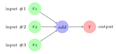
In TensorFlow, the add operation node in the preceding diagram would correspond to the code y = tf.add( x1 + x2 + x3 ).
The variables, constants, and placeholders get added to the graph as and when they are created. After defining the computation graph, a session object is instantiated that executes the operation objects and evaluates the tensor objects.
Let's define and execute a computation graph to calculate

, just like we saw in the preceding example:
# Linear Model y = w * x + b
# Define the model parameters
w = tf.Variable([.3], tf.float32)
b = tf.Variable([-.3], tf.float32)
# Define model input and output
x = tf.placeholder(tf.float32)
y = w * x + b
output = 0

with tf.Session() as tfs:
   # initialize and print the variable y
   tf.global_variables_initializer().run()
   output = tfs.run(y,{x:[1,2,3,4]})
print('output : ',output)
Creating and using a session in the with block ensures that the session is automatically closed when the block is finished. Otherwise, the session has to be explicitly closed with the tfs.close() command, where tfs is the session name.
The nodes in a computation graph are executed in their order of dependency. If node x depends on node y, then x is executed before y when the execution of y is requested. A node is only executed if either the node itself or another node depending on it is invoked for execution. This execution philosophy is known as lazy loading. As the name implies, the node objects are not instantiated and initialized until they are actually required.
Often, it is necessary to control the order of the execution of the nodes in a computation graph. This can be done with the tf.Graph.control_dependencies() function. For example, if the graph has the nodes l,m,n, and o, and we want to execute n and o before l and m, then we would use the following code:
with graph_variable.control_dependencies([n,o]):
  # other statements here
This makes sure that any node in the preceding with block is executed after nodes n and o have been executed.
A graph can be partitioned into several parts, and each part can be placed and executed on different devices, such as a CPU or GPU. All of the devices that are available for graph execution can be listed with the following command:
from tensorflow.python.client import device_lib
print(device_lib.list_local_devices())
The output is listed as follows (the output for your machine will be different because this will depend on the available compute devices in your specific system):
[name: "/device:CPU:0"
device_type: "CPU"
memory_limit: 268435456
locality {
}
incarnation: 12900903776306102093
, name: "/device:GPU:0"
device_type: "GPU"
memory_limit: 611319808
locality {
  bus_id: 1
}
incarnation: 2202031001192109390
physical_device_desc: "device: 0, name: Quadro P5000, pci bus id: 0000:01:00.0, compute capability: 6.1"
]
The devices in TensorFlow are identified with the string /device:<device_type>:<device_idx>. In the last output, CPU and GPU denote the device type, and 0 denotes the device index.
One thing to note about the last output is that it shows only one CPU, whereas our computer has 8 CPUs. The reason for this is that TensorFlow implicitly distributes the code across the CPU units and thus, by default, CPU:0 denotes all of the CPUs available to TensorFlow. When TensorFlow starts executing graphs, it runs the independent paths within each graph in a separate thread, with each thread running on a separate CPU. We can restrict the number of threads used for this purpose by changing the number of inter_op_parallelism_threads. Similarly, if, within an independent path, an operation is capable of running on multiple threads, TensorFlow will launch that specific operation on multiple threads. The number of threads in this pool can be changed by setting the number of intra_op_parallelism_threads.
To enable the logging of variable placement by defining a config object, set the log_device_placement property to true, and then pass this config object to the session as follows:
tf.reset_default_graph()

# Define model parameters
w = tf.Variable([.3], tf.float32)
b = tf.Variable([-.3], tf.float32)
# Define model input and output
x = tf.placeholder(tf.float32)
y = w * x + b

config = tf.ConfigProto()
config.log_device_placement=True

with tf.Session(config=config) as tfs:
# initialize and print the variable y
tfs.run(global_variables_initializer())
   print('output',tfs.run(y,{x:[1,2,3,4]}))
The output from the console window of the Jupyter Notebook is listed as follows:
b: (VariableV2): /job:localhost/replica:0/task:0/device:GPU:0
b/read: (Identity): /job:localhost/replica:0/task:0/device:GPU:0
b/Assign: (Assign): /job:localhost/replica:0/task:0/device:GPU:0
w: (VariableV2): /job:localhost/replica:0/task:0/device:GPU:0
w/read: (Identity): /job:localhost/replica:0/task:0/device:GPU:0
mul: (Mul): /job:localhost/replica:0/task:0/device:GPU:0
add: (Add): /job:localhost/replica:0/task:0/device:GPU:0
w/Assign: (Assign): /job:localhost/replica:0/task:0/device:GPU:0
init: (NoOp): /job:localhost/replica:0/task:0/device:GPU:0
x: (Placeholder): /job:localhost/replica:0/task:0/device:GPU:0
b/initial_value: (Const): /job:localhost/replica:0/task:0/device:GPU:0
Const_1: (Const): /job:localhost/replica:0/task:0/device:GPU:0
w/initial_value: (Const): /job:localhost/replica:0/task:0/device:GPU:0
Const: (Const): /job:localhost/replica:0/task:0/device:GPU:0
Thus, by default, TensorFlow creates the variable and operations nodes on a device so that it can get the highest performance. These variables and operations can be placed on specific devices by using the tf.device() function. Let's place the graph on the CPU:
tf.reset_default_graph()

with tf.device('/device:CPU:0'):
# Define model parameters
w = tf.get_variable(name='w',initializer=[.3], dtype=tf.float32)
    b = tf.get_variable(name='b',initializer=[-.3], dtype=tf.float32)
# Define model input and output
x = tf.placeholder(name='x',dtype=tf.float32)
    y = w * x + b

config = tf.ConfigProto()
config.log_device_placement=True

with tf.Session(config=config) as tfs:
# initialize and print the variable y
tfs.run(tf.global_variables_initializer())
   print('output',tfs.run(y,{x:[1,2,3,4]}))
In the Jupyter console, we can see that the variables have been placed on the CPU and that execution also takes place on the CPU:
b: (VariableV2): /job:localhost/replica:0/task:0/device:CPU:0
b/read: (Identity): /job:localhost/replica:0/task:0/device:CPU:0
b/Assign: (Assign): /job:localhost/replica:0/task:0/device:CPU:0
w: (VariableV2): /job:localhost/replica:0/task:0/device:CPU:0
w/read: (Identity): /job:localhost/replica:0/task:0/device:CPU:0
mul: (Mul): /job:localhost/replica:0/task:0/device:CPU:0
add: (Add): /job:localhost/replica:0/task:0/device:CPU:0
w/Assign: (Assign): /job:localhost/replica:0/task:0/device:CPU:0
init: (NoOp): /job:localhost/replica:0/task:0/device:CPU:0
x: (Placeholder): /job:localhost/replica:0/task:0/device:CPU:0
b/initial_value: (Const): /job:localhost/replica:0/task:0/device:CPU:0
Const_1: (Const): /job:localhost/replica:0/task:0/device:CPU:0
w/initial_value: (Const): /job:localhost/replica:0/task:0/device:CPU:0
Const: (Const): /job:localhost/replica:0/task:0/device:CPU:0TensorFlow follows the following rules for placing the variables on devices:
If the graph was previously run,
    then the node is left on the device where it was placed earlier
Else If the tf.device() block is used,
    then the node is placed on the specified device
Else If the GPU is present
    then the node is placed on the first available GPU
Else If the GPU is not present
then the node is placed on the CPUThe tf.device() function can be provided with a function name in place of a device string. If a function name is provided, then the function has to return the device string. This way of providing a device string through a custom function allows complex algorithms to be used for placing the variables on different devices. For example, TensorFlow provides a round robin device setter function in tf.train.replica_device_setter().
If a TensorFlow operation is placed on the GPU, then the execution engine must have the GPU implementation of that operation, known as the kernel. If the kernel is not present, then the placement results in a runtime error. Also, if the requested GPU device does not exist, then a runtime error is raised. The best way to handle such errors is to allow the operation to be placed on the CPU if requesting the GPU device results in an error. This can be achieved by setting the following config value:
config.allow_soft_placement = True
At the start of the TensorFlow session, by default, a session grabs all of the GPU memory, even if the operations and variables are placed only on one GPU in a multi-GPU system. If another session starts execution at the same time, it will receive an out-of-memory error. This can be solved in multiple ways:
- For multi-GPU systems, set the environment variable
CUDA_VISIBLE_DEVICES=<list of device idx>:
os.environ['CUDA_VISIBLE_DEVICES']='0'
The code that's executed after this setting will be able to grab all of the memory of the visible GPU.
- For letting the session grab a part of the memory of the GPU, use the config option
per_process_gpu_memory_fractionto allocate a percentage of the memory:
config.gpu_options.per_process_gpu_memory_fraction = 0.5
This will allocate 50% of the memory in all of the GPU devices.
- By combining both of the preceding strategies, you can make only a certain percentage, alongside just some of the GPU, visible to the process.
- Limit the TensorFlow process to grab only the minimum required memory at the start of the process. As the process executes further, set a config option to allow for the growth of this memory:
config.gpu_options.allow_growth = True
This option only allows for the allocated memory to grow, so the memory is never released back.
We can create our own graphs, which are separate from the default graph, and execute them in a session. However, creating and executing multiple graphs is not recommended, because of the following disadvantages:
- Creating and using multiple graphs in the same program would require multiple TensorFlow sessions, and each session would consume heavy resources
- Data cannot be directly passed in-between graphs
Hence, the recommended approach is to have multiple subgraphs in a single graph. In case we wish to use our own graph instead of the default graph, we can do so with the tf.graph() command. In the following example, we create our own graph, g, and execute it as the default graph:
g = tf.Graph()
output = 0

# Assume Linear Model y = w * x + b

with g.as_default():
 # Define model parameters
 w = tf.Variable([.3], tf.float32)
 b = tf.Variable([-.3], tf.float32)
 # Define model input and output
 x = tf.placeholder(tf.float32)
 y = w * x + b

with tf.Session(graph=g) as tfs:
 # initialize and print the variable y
 tf.global_variables_initializer().run()
 output = tfs.run(y,{x:[1,2,3,4]})

print('output : ',output)
Now, let's put this learning into practice and implement the classification of handwritten digital images with TensorFlow.
Let's now learn about machine learning, classification, and logistic regression.
Machine learning refers to the application of algorithms to make computers learn from data. The models that are learned by computers are used to make predictions and forecasts. Machine learning has been successfully applied in a variety of areas, such as natural language processing, self-driving vehicles, image and speech recognition, chatbots, and computer vision.
Machine learning algorithms are broadly categorized into three types:
- Supervised learning: In supervised learning, the machine learns the model from a training dataset that consists of features and labels. The supervised learning problems are generally of two types: regression and classification. Regression refers to predicting future values based on the model, while classification refers to predicting the categories of the input values.
- Unsupervised learning: In unsupervised learning, the machine learns the model from a training dataset that consists of features only. One of the most common types of unsupervised learning is known as clustering. Clustering refers to dividing the input data into multiple groups, thus producing clusters or segments.
- Reinforcement learning: In reinforcement learning, the agent starts with an initial model and then continuously learns the model based on the feedback from the environment. A reinforcement learning agent learns or updates the model by applying supervised or unsupervised learning techniques as part of the reinforcement learning algorithms.
These machine learning problems are abstracted to the following equation in one form or another:

Here, y represents the target and x represents the feature. If x is a collection of features, it is also called a feature vector and denoted with X. The model is the function f that maps features to targets. Once the computer learns f, it can use the new values of x to predict the values of y.
The preceding simple equation can be rewritten in the context of linear models for machine learning as follows:

Here, w is known as the weight and b is known as the bias. Thus, the machine learning problem now can be stated as a problem of finding w and b from the current values of X so that the equation can now be used to predict the values of y.
Regression analysis or regression modeling refers to the methods and techniques used to estimate relationships among variables. The variables that are used as input for regression models are called independent variables, predictors, or features, and the output variables from regression models are called dependent variables or targets. Regression models are defined as follows:

Where Y is the target variable, X is a vector of features, and β is a vector of parameters (w,b in the preceding equation).
Classification is one of the classical problems in machine learning. Data under consideration could belong to one class or another, for example, if the images provided are data, they could be pictures of cats or dogs. Thus, the classes, in this case, are cats and dogs. Classification means identifying the label or class of the objects under consideration. Classification falls under the umbrella of supervised machine learning. In classification problems, a training dataset is provided that has features or inputs and their corresponding outputs or labels. Using this training dataset, a model is trained; in other words, the parameters of the model are computed. The trained model is then used on new data to find its correct labels.
Classification problems can be of two types: binary class or multiclass. Binary class means that the data is to be classified into two distinct and discrete labels; for example, the patient has cancer or the patient does not have cancer, and the images are of cats or dogs and so on. Multiclass means that the data is to be classified among multiple classes, for example, an email classification problem will divide emails into social media emails, work-related emails, personal emails, family-related emails, spam emails, shopping offer emails, and so on. Another example would be of pictures of digits; each picture could be labeled between 0 and 9, depending on what digit the picture represents. In this chapter, we will look at examples of both kinds of classification.
The most popular method for classification is logistic regression. Logistic regression is a probabilistic and linear classifier. The probability that the vector of input features belongs to a specific class can be described mathematically by the following equation:

In the preceding equation, the following applies:
- Y represents the output
- i represents one of the classes
- x represents the inputs
- w represents the weights
- b represents the biases
- z represents the regression equation

- ϕ represents the smoothing function (or model, in our case)
The ϕ(z) function represents the probability that x belongs to class i when w and b are given. Thus, the model has to be trained to maximize the value of this probability.
For binary classification, the model function ϕ(z) is defined as the sigmoid function, which can be described as follows:

The sigmoid function transforms the y value to be between the range [0,1]. Thus, the value of y=ϕ(z) can be used to predict the class: if y > 0.5, then the object belongs to 1, otherwise the object belongs to 0.
The model training means to search for the parameters that minimize the loss function, which can either be the sum of squared errors or the sum of mean squared errors. For logistic regression, the likelihood is maximized as follows:

However, as it is easier to maximize the log-likelihood, we use the log-likelihood (l(w)) as the cost function. The loss function (J(w)) is written as -l(w), and can be minimized by using optimization algorithms such as gradient descent.
The loss function for binary logistic regression is written mathematically as follows:

Here, ϕ(z) is the sigmoid function.
When more than two classes are involved, logistic regression is knownas multinomial logistic regression. In multinomial logistic regression, instead of sigmoid, use the softmax function, which can be described mathematically as follows:

The softmax function produces the probabilities for each class so that the probabilities vector adds up to 1. At the time of inference, the class with the highest softmax value becomes the output or predicted class. The loss function, as we discussed earlier, is the negative log-likelihood function, -l(w), that can be minimized by the optimizers, such as gradient descent.
The loss function for multinomial logistic regression is written formally as follows:

Here, ϕ(z) is the softmax function.
We will implement this loss function in the next section. In the following section, we will dig into our example for multiclass classification with logistic regression in TensorFlow.
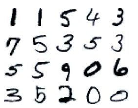
One of the most popular examples regarding multiclass classification is to label the images of handwritten digits. The classes, or labels, in this example are {0,1,2,3,4,5,6,7,8,9}. The dataset that we are going to use is popularly known as MNIST and is available from the following link: http://yann.lecun.com/exdb/mnist/. The MNIST dataset has 60,000 images for training and 10,000 images for testing. The images in the dataset appear as follows:
- First, we must import
datasetslib, a library that was written by us to help with examples in this book (available as a submodule of this book's GitHub repository):
DSLIB_HOME = '../datasetslib'
import sys
if not DSLIB_HOME in sys.path:
    sys.path.append(DSLIB_HOME)
%reload_ext autoreload
%autoreload 2
import datasetslib as dslib

from datasetslib.utils import imutil
from datasetslib.utils import nputil
from datasetslib.mnist import MNIST- Set the path to the
datasetsfolder in our home directory, which is where we want all of thedatasetsto be stored:
import os
datasets_root = os.path.join(os.path.expanduser('~'),'datasets')- Get the MNIST data using our
datasetsliband print the shapes to ensure that the data is loaded properly:
mnist=MNIST()

x_train,y_train,x_test,y_test=mnist.load_data()

mnist.y_onehot = True
mnist.x_layout = imutil.LAYOUT_NP
x_test = mnist.load_images(x_test)
y_test = nputil.onehot(y_test)

print('Loaded x and y')
print('Train: x:{}, y:{}'.format(len(x_train),y_train.shape))
print('Test: x:{}, y:{}'.format(x_test.shape,y_test.shape))- Define the hyperparameters for training the model:
learning_rate = 0.001
n_epochs = 5
mnist.batch_size = 100
- Define the placeholders and parameters for our simple model:
# define input images
x = tf.placeholder(dtype=tf.float32, shape=[None, mnist.n_features])
# define output labels
y = tf.placeholder(dtype=tf.float32, shape=[None, mnist.n_classes])

# model parameters
w = tf.Variable(tf.zeros([mnist.n_features, mnist.n_classes]))
b = tf.Variable(tf.zeros([mnist.n_classes]))
- Define the model with
logitsandy_hat:
logits = tf.add(tf.matmul(x, w), b)
y_hat = tf.nn.softmax(logits)
- Define the
lossfunction:
epsilon = tf.keras.backend.epsilon()
y_hat_clipped = tf.clip_by_value(y_hat, epsilon, 1 - epsilon)
y_hat_log = tf.log(y_hat_clipped)
cross_entropy = -tf.reduce_sum(y * y_hat_log, axis=1)
loss_f = tf.reduce_mean(cross_entropy)
- Define the
optimizerfunction:
optimizer = tf.train.GradientDescentOptimizer
optimizer_f = optimizer(learning_rate=learning_rate).minimize(loss_f)
- Define the function to check the accuracy of the trained model:
predictions_check = tf.equal(tf.argmax(y_hat, 1), tf.argmax(y, 1))
accuracy_f = tf.reduce_mean(tf.cast(predictions_check, tf.float32))
- Run the
trainingloop for each epoch in a TensorFlow session:
n_batches = int(60000/mnist.batch_size)

with tf.Session() as tfs:
    tf.global_variables_initializer().run()
for epoch in range(n_epochs):
        mnist.reset_index()
for batch in range(n_batches):
            x_batch, y_batch = mnist.next_batch()
            feed_dict={x: x_batch, y: y_batch}
            batch_loss,_ = tfs.run([loss_f, optimizer_f],feed_dict=feed_dict )
#print('Batch loss:{}'.format(batch_loss))
- Run the evaluation function for each epoch with the test data in the same TensorFlow session that was created previously:
feed_dict = {x: x_test, y: y_test}
accuracy_score = tfs.run(accuracy_f, feed_dict=feed_dict)
print('epoch {0:04d}  accuracy={1:.8f}'
.format(epoch, accuracy_score))
We get the following output:
epoch 0000 accuracy=0.73280001 epoch 0001 accuracy=0.72869998 epoch 0002 accuracy=0.74550003 epoch 0003 accuracy=0.75260001 epoch 0004 accuracy=0.74299997
There you go. We just trained our very first logistic regression model using TensorFlow for classifying handwritten digit images and got 74.3% accuracy.
Now, let's see how writing the same model in Keras makes this process even easier.
Keras is a high-level library that is available as part of TensorFlow. In this section, we will rebuild the same model we built earlier with TensorFlow core with Keras:
- Keras takes data in a different format, and so we must first reformat the data using
datasetslib:
x_train_im = mnist.load_images(x_train)

x_train_im, x_test_im = x_train_im / 255.0, x_test / 255.0
In the preceding code, we are loading the training images in memory before both the training and test images are scaled, which we do by dividing them by 255.
- Then, we build the model:
model = tf.keras.models.Sequential([
    tf.keras.layers.Flatten(),
    tf.keras.layers.Dense(10, activation=tf.nn.softmax)
])- Compile the model with the
sgdoptimizer. Set the categorical entropy as thelossfunction and the accuracy as a metric to test the model:
model.compile(optimizer='sgd',
loss='sparse_categorical_crossentropy',
metrics=['accuracy'])
- Train the model for
5epochs with the training set of images and labels:
model.fit(x_train_im, y_train, epochs=5)

Epoch 1/5
60000/60000 [==============================] - 3s 45us/step - loss: 0.7874 - acc: 0.8095
Epoch 2/5
60000/60000 [==============================] - 3s 42us/step - loss: 0.4585 - acc: 0.8792
Epoch 3/5
60000/60000 [==============================] - 2s 42us/step - loss: 0.4049 - acc: 0.8909
Epoch 4/5
60000/60000 [==============================] - 3s 42us/step - loss: 0.3780 - acc: 0.8965
Epoch 5/5
60000/60000 [==============================] - 3s 42us/step - loss: 0.3610 - acc: 0.9012
10000/10000 [==============================] - 0s 24us/step
- Evaluate the model with the test data:
model.evaluate(x_test_im, nputil.argmax(y_test))
We get the following evaluation scores as output:
[0.33530342621803283, 0.9097]Wow! Using Keras, we can achieve higher accuracy. We achieved approximately 90% accuracy. This is because Keras internally sets many optimal values for us so that we can quickly start building models.
In this chapter, we briefly covered the TensorFlow library. We covered the TensorFlow data model elements, such as constants, variables, and placeholders, and how they can be used to build TensorFlow computation graphs. We learned how to create tensors from Python objects. Tensor objects can also be generated as specific values, sequences, or random valued distributions from various TensorFlow library functions.
We covered the TensorFlow programming model, which includes defining and executing computation graphs. These computation graphs have nodes and edges. The nodes represent operations and edges represent tensors that transfer data from one node to another. We covered how to create and execute graphs, the order of execution, and how to execute graphs on multiple compute devices, such as CPU and GPU.
We also learned about machine learning and implemented a classification algorithm to identify the handwritten digits dataset. The algorithm we implemented is known as multinomial logistic regression. We used both TensorFlow core and Keras to implement the logistic regression algorithm.
Starting from the next chapter, we will look at many projects that will be implemented using TensorFlow and Keras.
Enhance your understanding by practicing the following questions:
- Modify the logistic regression model that was given in this chapter so that you can use different training rates and observe how it impacts training
- Use different optimizer functions and observe the impact of different functions on training time and accuracy
We suggest the reader learn more by reading the following materials:
- Mastering TensorFlow by Armando Fandango.
- TensorFlow tutorials at https://www.tensorflow.org/tutorials/.
TensorFlow 1.x Deep Learning Cookbook by Antonio Gulli and Amita Kapoor