


 Download code from GitHub
Faster and efficient information retrieval is the primary objective of most computer programs. Data structures and algorithms help us in achieving the objective by processing and retrieving data faster. Information retrieval can easily be integrated with algorithms to answer inferential questions from data such as:
How are sales increasing over time?
What is customer's arrival distribution over time?
Out of all the customers who visit between 3:00 and 6:00 PM, how many order Asian versus Chinese?
Of all the customers visiting, how many are from the same city?
In the efficient processing of the preceding queries, especially in big data scenarios, data structures and algorithms utilized for data retrieval play a significant role. This book will introduce primary data structures such as lists, queues, and stacks, which are used for information retrieval and trade-off of different data structures. We will also introduce the data structure and algorithms evaluation approach for retrieval and processing of defined data structures.
Algorithms are evaluated based on complexity and efficiency, where complexity refers to an algorithm design which is easy to program and debug, and efficacy ensures that the algorithm is utilizing computer resources optimally. This book will focus on the efficiency part of algorithms using data structures, and the current chapter introduces the importance of data structure and the algorithms used for retrieval of data from data structures.
Moore's law in 1965 observed that the number of transistors per square inch in a dense integrated circuit (IC) had doubled every year since its invention, thus enhancing computational power per computer. He revised his forecast in 1975, stating that the number of transistors would double every 2 years, instead of every year, due to saturation:
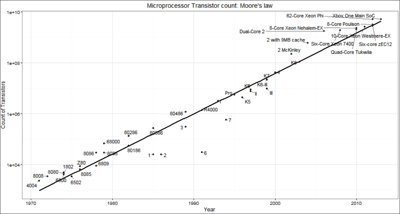
Figure 1.1: Moore's law (Ref: data credit - Transistor count, Wikipedia)
Also, although the computational power has been increasing, problem complexity and data sources have also been increasing exponentially over the decade, enforcing the need for efficient algorithms:
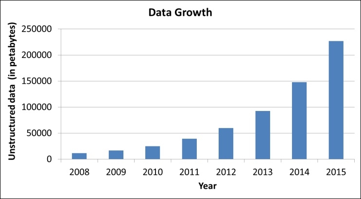
Figure 1.2: Increase in size of unstructured data (Ref: Enterprise strategy group 2010)
This explosion in data from 2008 to 2015 has led to a new field of data science where people put in a lot of effort to derive insights using all kinds of datasets such as structured, semi-structured, and unstructured. Thus, to efficiently deal with data scalability, it is important to efficiently store and retrieve datasets. For example, searching for a word in a dictionary would take a long time if the data is randomly organized; thus, sorted list data structures are utilized to ensure a faster search of words. Similarly, searching for an optimal path in a city based on the input location requires data about road network, position, and so on to be stored in the form of geometries. Ideally, even a variable stored as any built-in data type such as character, integer, or float can be considered as a data structure of scalar nature. However, data structure is formally defined as a scheme of organizing related information in a computer so that it can be used efficiently.
Similarly, for algorithms, given sufficient space and time, any dataset can be stored and processed to answer questions of interest. However, selecting the correct data structure will help you save a lot of memory and computational power. For example, assigning a float to integer data type, such as the number of customers coming in a day, will require double the memory. However, in the real-world scenario, computers are constrained by computational resources and space. Thus, a solution can be stated as efficient if it is able to achieve the desired goal in the given resources and time. Thus, this could be used as a cost function to compare the performance of different data structures while designing algorithms. There are two major design constraints to be considered while selecting the data structure:
Analyze the problem to decide on the basic operation that must be supported into the selected data structure, such as inserting an item, deleting an item, and searching for an item
Evaluate the resource constraint for each operation
The data structure is selected depending on the problem scenario, for example, a case where complete data is loaded at the beginning, and there is no change/insertion in data, requires similar data structure. However, similar including deletion into data structure will make data structure implementation more complex.
Tip
Detailed steps to download the code bundle are mentioned in the Preface of this book. Please have a look. The code bundle for the book is also hosted on GitHub at https://github.com/PacktPublishing/R-Data-Structures-and-Algorithms. We also have other code bundles from our rich catalog of books and videos available at https://github.com/PacktPublishing/. Check them out!
The abstract data type (ADT) is used to define high-level features and operations for data structure, and is required before we dig down into details of implementation of data structure. For example, before implementing a linked list, it would be good to know what we want to do with the defined linked list, such as:
I should be able to insert an item into the linked list
I should be able to delete an item from the linked list
I should be able to search an item in the linked list
I should be able to see whether the linked list is empty or not
The defined ADT will then be utilized to define the implementation strategy. We will discuss ADT for different data structures in more detail later in this book. Before getting into definitions of ADT, it's important to understand data types and their characteristics, as they will be utilized to build an ecosystem for the data structures.
Data type is a way to classify various types of data such as Boolean, integer, float, and string. To efficiently classify a dataset, the following characteristics are needed in any data type:
Atomic: It should define a single concept
Traceable: It should be able to map with the same data type
Accurate: It should be unambiguous
Clear and concise: It should be understandable
Data types can be classified into two types:
Built-in data type
Derived data type
Data types for which a language has built-in support are known as built-in data types. For example, R supports the following data types:
Integers
Float
Boolean
Character
Data types which are obtained by integrating the built-in data types with associated operations such as insertion, deletion, sorting, merging, and so on are referred to as derived data types, such as:
List
Array
Stack
Queue
Derived data types or data structures are studied on two components:
Abstract data type or mathematical/logical models
Programming implementation
ADT is the realization of a data type in software. In ADT, we usually look into high-level features and operations used by users for a data structure, but do not know how these features run in the background. For example, say a user using banking software with search functionality is searching for the transaction history of Mr. Smith, using the search feature of the software. The user does not have any idea about the operations performed, or the implementation details of the data structures. Thus, the behavior of ADT is managed by input and output only:
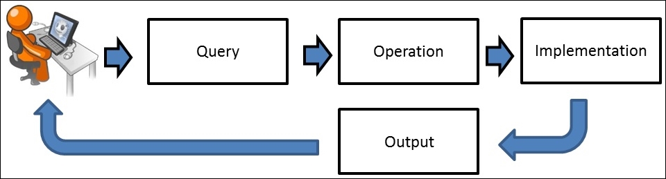
Figure 1.3: Framework for ADT
Thus, ADT does not know how the data type is implemented, as these details are hidden by the user and protected from outside access, a concept referred to as encapsulation. A data structure is the implementation part of ADT, which can be implemented in any programming language. ADT can be achieved by multiple implementation strategies, as shown in Figure 1.4:
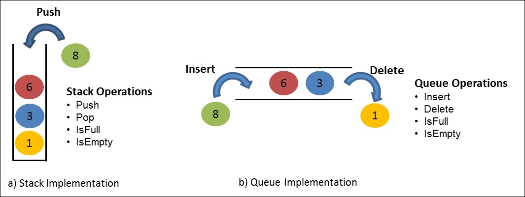
Figure 1.4: Illustration of stack and queue implementation using array with integer data type
The abstraction provided by ADT helps to manage programming complexity. The ADT is also referred to as logical form, as it decides the type and operations required for implementation. The ADT is implemented by using a particular type of data structure. The data structure used to implement ADT is referred to as the physical form of data type, as it manages storage using the implementation subroutine.
Problem can be defined as the task to be performed. The execution of the task to be performed can be divided primarily into two components:
Data
Algorithm
However, there could be other controlling factors which could affect your approach development, such as problem constraints, resource constraints, computation time allowed, and so on.
The data component of the problem represents the information we are dealing with, such as numbers, text, files, and so on. For example, let's assume we want to maintain the company employee records, which include the employee name and their associated work details. This data needs to be maintained and updated regularly.
The algorithm part of a problem represents more of implementation details. It entails how we are going to manage the current data. Depending on the data and problem requirements, we select the data structure. Depending on the data structure, we have to define the algorithm to manage the dataset. For example, we can store the company employees dataset into a linked list or dictionary. Based on the defined data structure to store data approach for searching, insertion, and deletion and so on operations performed on data structure changes which is control by algorithms and implemented as program. Thus, we could state that a program is the step-by-step instructions given to a computer to do some operations:
Program = f(Algorithm, Data Structure)
To summarize, we could state that a program is the group of step-by-step instructions to solve a defined problem using the algorithm selected considering all problems and resource constraints. This book will use program representations using R to demonstrate the implementation of different data structures and algorithms.
R is a statistical programming language designed and created by Ross Ihaka and Robert Gentleman. It is a derivative of the S language created at the AT&T Bell laboratories. Apart from statistical analysis, R also supports powerful visualizations. It is open source, freely distributed under a General Public License (GPL). Comprehensive R Archive Network (CRAN) is an ever-growing repository with more than 8,400 packages, which can be freely installed and used for various kinds of analysis.
R is a high-level language based on interpretations and intuitive syntax. It runs on system's or server's active memory (RAM) and stores all files, functions, and derived results in its environment as objects. The architecture utilized in R computation is shown in Figure 1.5:
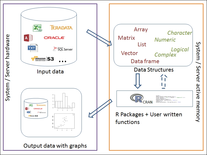
Figure 1.5: Illustrate architecture of R in local/server mode
R can be installed on any operating system, such as Windows, Mac OS X, and Linux. The installation files of the most recent version can be downloaded from any one of the mirror sites of CRAN: https://cran.r-project.org/. It is available under both 32-bit and 64-bit architectures.
The installation of r-base-dev is also highly recommended as it has many built-in functions. It also enables us to install and compile new R packages directly from the R console using the install.packages() command.
Upon installation, R can be called from program files, desktop shortcut, or from the command line. With default settings, the R console looks as follows:
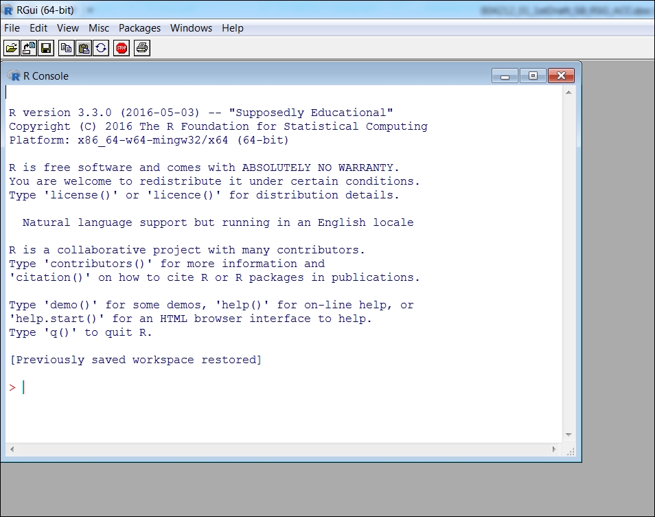
Figure 1.6: The R console in which one can start coding and evaluate results instantly
R can also be used as a kernel within Jupyter Notebook. Jupyter Notebook is a web-based application that allows you to combine documentation, output, and code. Jupyter can be installed using pip:
pip3 install -upgrade pip
pip3 install jupyter
To start Jupyter Notebook, open a shell/terminal and run this command to start the Jupyter Notebook interface in your browser:
jupyter notebook
To start a new R Notebook, click on right hand side New tab and select R kernel as shown in Figure 1.7. R kernel does not come as default in Jupyter Notebook with Python as prerequisite. Anaconda distribution is recommended to install python and Jupyter and can be downloaded from https://www.continuum.io/downloads. R essentials can be installed using below command.
conda install -c r r-essentials
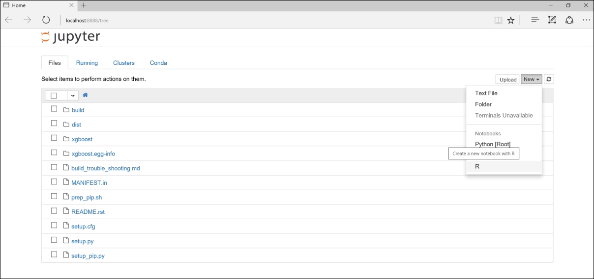
Figure 1.7: Jupyter Notebook for creating R notebooks
Once notebook is opened, you could start organizing your code into cells. As R does not require formal compilation, and executes codes on runtime, one can start coding and evaluate instant results. The console view can be modified using some options under the Windows tab. However, it is highly recommended to use an Integrated Development Environment (IDE), which would provide a powerful and productive user interface for R. One such widely used IDE is RStudio, which is free and open source. It comes with its own server (RStudio Server Pro) too. The interface of RStudio is as seen in the following screenshot:
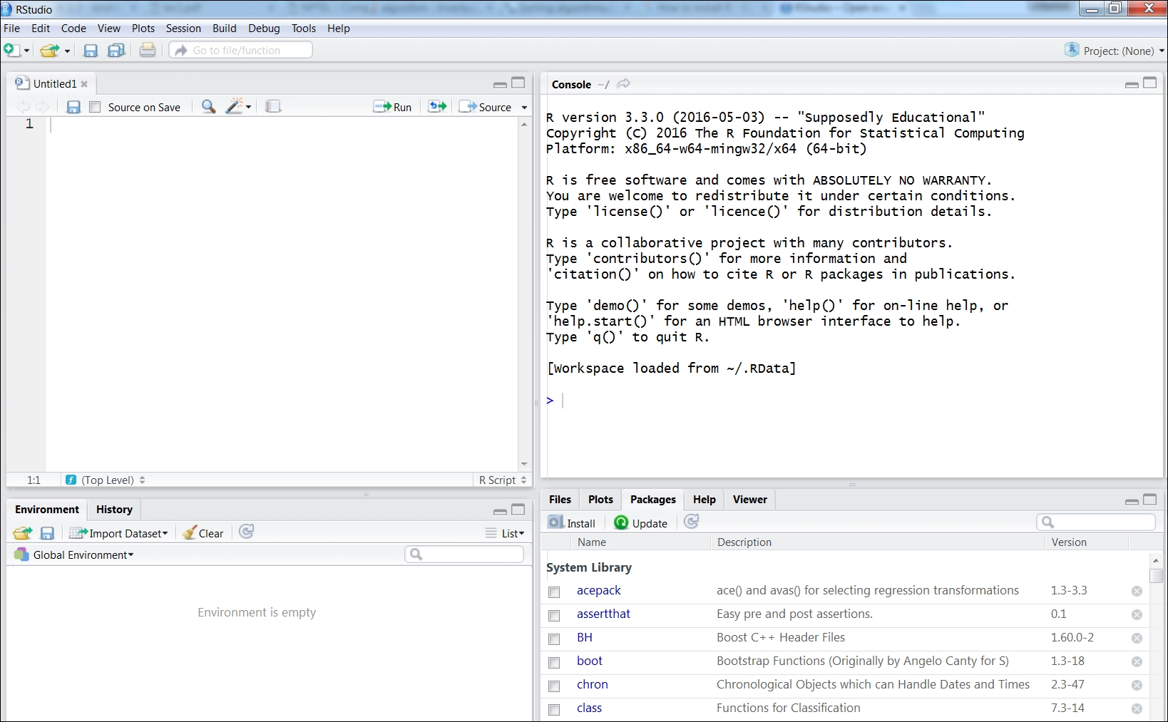
Figure 1.8: RStudio, a widely used IDE for R
R supports multiple types of data, which can be organized by dimensions and content type (homogeneous or heterogeneous), as shown in Table 1.1:
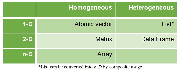
Table 1.1 Basic data structure in R
Homogeneous data structure is one which consists of the same content type, whereas heterogeneous data structure supports multiple content types. All other data structures, such as data tables, can be derived using these foundational data structures. Data types and their properties will be covered in detail in Chapter 3, Linked Lists.
The syntax of operators in R is very similar to other programming languages. The following is a list of operators along with their explanations.
The following table defines the various arithmetic operators:
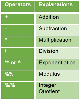
Table 1.2 Basic arithmetic operators in R
The following table defines the various logical operators:
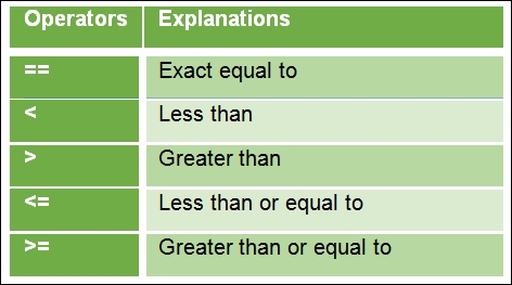
Table 1.3 Basic logical operators in R
An example of assigned in R is shown below. Initially a column vector V is assigned followed by operations on column vector such as addition, subtraction, square root and log. Any operation applied on column vector is element-wise operation.
> V <- c(1,2,3,4,5,6)  ## Assigning a vector V
> V
[1] 1 2 3 4 5 6
> V+10 ## Adding each element in vector V with 10
[1] 11 12 13 14 15 16
> V-1  ## Subtracting each element in vector V with 1
[1] 0 1 2 3 4 5
> sqrt(V)  ## Performing square root operation on each element in  vector V
[1] 1.000000 1.414214 1.732051 2.000000 2.236068 2.449490
> V1 <- log(V)  ## Storing log transformed of vector V as V1
> V1
[1] 0.0000000 0.6931472 1.0986123 1.3862944 1.6094379 1.7917595
Control structures such as loops and conditions form an integral part of any programming language, and R supports them with much intuitive syntax.
The syntax for the if condition is as follows:
    if (test expression)
    {
      Statement upon condition is true
    }
If the test expression is true, the statement is executed. If the statement is false, nothing happens.
In the following example, an atomic vector x is defined, and it is subjected to two conditions separately, that is, whether x is greater than 5 or less than 5. If either of the conditions gets satisfied, the value x gets printed in the console following the corresponding if statement:
> x <- 10
> if (x < 5) print(x)
> if (x > 5) print(x)
[1] 10
The syntax for the if...else condition is as follows:
    if(test expression)
    {
      Statement upon condition is true
    } else {
      Statement upon condition is false
    }
In this scenario, if the condition in the test expression is true, the statement under the if condition is executed, otherwise the statement under the else condition is executed.
The following is an example in which we define an atomic vector x with a value 10. Then, we verify whether x, when divided by 2, returns 1 (R reads 1 as a Boolean True). If it is True, the value x gets printed as an odd number, else as an even number:
> x=10
> if (x %% 2)
+ {
+   print(paste0(x, " :odd number"))
+ } else {
+   print(paste0(x, " :even number"))
+ }
[1] "10 :even number"
An ifelse() function is a condition used primarily for vectors, and it is an equivalent form of the if...else statement. Here, the conditional function is applied to each element in the vector individually. Hence, the input to this function is a vector, and the output obtained is also a vector. The following is the syntax of the ifelse condition:
    ifelse (test expression, statement upon condition is true,
    statement upon condition is false)
In this function, the primary input is a test expression which must provide a logical output. If the condition is true, the subsequent statement is executed, else the last statement is executed.
The following is example in which a vector x is defined with integer values from 1 to 7. Then, a condition is applied on each element in vector x to determine whether the element is an odd number or an even number:
> x <- 1:6
> ifelse(x %% 2, paste0(x, " :odd number"), paste0(x, " :even  number"))
[1] "1 :odd number"  "2 :even number" "3 :odd number"
[4] "4 :even number" "5 :odd number"  "6 :even number"
A for loop is primarily used to iterate a statement over a vector of values in a given sequence. The vector can be of any type, that is, numeric, character, Boolean, or complex. For every iteration, the statement is executed.
The following is the syntax of the for loop:
    for(x in sequence vector)
    {
      Statement to be iterated
    }
The loop continues till all the elements in the vector get exhausted as per the given sequence.
The following example details a for loop. Here, we assign a vector x, and each element in vector x is printed in the console using a for loop:
> x <- c("John", "Mary", "Paul", "Victoria")
> for (i in seq(x)) {
+   print(x[i])
+ }
[1] "John"
[1] "Mary"
[1] "Paul"
[1] "Victoria"
The nested for loop can be defined as a set of multiple for loops within each for loop as shown here:
    for( x in sequence vector)
    {
      First statement to be iterated
      for(y in sequence vector)
    {
      Second statement to be iterated
      .........
    }
  }
In a nested for loop, each subsequent for loop is iterated for all the possible times based on the sequence vector in the previous for loop. This can be explained using the following example, in which we define mat as a matrix (3x3), and our desired objective is to obtain a series of summations which will end up with the total sum of all the values within the matrix. Firstly, we initialize sum to 0, and then subsequently, sum gets updated by adding itself to all the elements in the matrix in a sequence. The sequence is defined by the nested for loop, wherein for each row in a matrix, each of the values in all the columns gets added to sum:
> mat <- matrix(1:9, ncol = 3)
> sum <- 0
> for (i in seq(nrow(mat)))
+ {
+   for (j in seq(ncol(mat)))
+   {
+     sum <- sum + mat[i, j]
+     print(sum)
+   }
+ }
[1] 1
[1] 5
[1] 12
[1] 14
[1] 19
[1] 27
[1] 30
[1] 36
[1] 45
In R, while loops are iterative loops with a specific condition which needs to be satisfied. The syntax of the while loop is as follows:
    while (test expression)
   {
     Statement upon condition is true (iteratively)
   }
Let's understand the while loop in detail with an example. Here, an object i is initialized to 1. The test expression which needs to be satisfied for every iteration is i<10. Since i = 1, the condition is TRUE, and the statement within the while loop is evaluated. According to the statement, i is printed on the console, and then increased by 1 unit. Now i increments to 2, and once again, the test expression, whether the condition (i < 10) is true or false, is checked. If TRUE, the statement is again evaluated. The loop continues till the condition becomes false, which, in our case, will happen when i increments to 10. Here, incrementing i becomes very critical, without which the loop can turn into infinite iterations:
> i <- 1
> while (i < 10)
+ {
+   print(i)
+   i <- i + 1
+ }
[1] 1
[1] 2
[1] 3
[1] 4
[1] 5
[1] 6
[1] 7
[1] 8
[1] 9
In R, the loops can be altered using break or next statements. This helps in inducing other conditions required within the statement inside the loop.
The syntax for the Break statement is break. It is used to terminate a loop and stop the remaining iterations. If a break statement is provided within a nested loop, then the innermost loop within which the break statement is mentioned gets terminated, and iterations of the outer loops are not affected.
The following is an example in which a for loop is terminated when i reaches the value 8:
> for (i in 1:30)
+ {
+   if (i < 8)
+   {
+     print(paste0("Current value is ",i))
+   } else {
+     print(paste0("Current value is ",i," and the loop breaks"))
+     break
+   }
+ }
[1] "Current value is 1"
[1] "Current value is 2"
[1] "Current value is 3"
[1] "Current value is 4"
[1] "Current value is 5"
[1] "Current value is 6"
[1] "Current value is 7"
[1] "Current value is 8 and the loop breaks"
The syntax for a Next statement is next. The next statements are used to skip intermediate iterations within a loop based on a condition. Once the condition for the next statement is met, all the subsequent operations within the loop get terminated, and the next iteration begins.
This can be further explained using an example in which we print only odd numbers based on a condition that the printed number, when divided by 2, leaves the remainder 1.
> for (i in 1:10)
+ {
+   if (i %% 2)
+   {
+     print(paste0(i, " is an odd number."))
+   } else {
+     next
+   }
+ }
[1] "1 is an odd number."
[1] "3 is an odd number."
[1] "5 is an odd number."
[1] "7 is an odd number."
[1] "9 is an odd number."
The repeat loop is an infinite loop which iterates multiple times without any inherent condition. Hence, it becomes mandatory for the user to explicitly mention the terminating condition, and use a break statement to terminate the loop.
The following is the syntax for a repeat statement:
    repeat
    {
      Statement to iterate along with explicit terminate condition
      including break statement
    }
In the current example, i is initialized to 1. Then, a for loop iterates, within which an object cube is evaluated and verified using a condition whether the cube is greater than 729 or not. Simultaneously, i is incremented by 1 unit. Once the condition is met, the for loop is terminated using a break statement:
> i <- 1
> repeat
+ {
+   cube <- i ** 3
+   i <- i + 1
+   if (cube < 729)
+   {
+     print(paste0(cube, " is less than 729. Let's remain in the
      loop."))
+   } else {
+     print(paste0(cube, " is greater than or equal to 729. Let's exit
      the loop."))
+     break
+   }
+ }
[1] "1 is less than 729. Let's remain in the loop."
[1] "8 is less than 729. Let's remain in the loop."
[1] "27 is less than 729. Let's remain in the loop."
[1] "64 is less than 729. Let's remain in the loop."
[1] "125 is less than 729. Let's remain in the loop."
[1] "216 is less than 729. Let's remain in the loop."
[1] "343 is less than 729. Let's remain in the loop."
[1] "512 is less than 729. Let's remain in the loop."
[1] "729 is greater than 729. Let's exit the loop."
R is primarily a functional language at its core. In R, functions are treated just like any other data types, and are considered as first-class citizens. The following example shows that R considers everything as a function call.
Here, the operator + is a function in itself:
> 10+20
[1] 30
> "+"(10,20)
[1] 30
Here, the operator ^ is also a function in itself:
> 4^2
[1] 16
> "^"(4,2)
[1] 16
Now, let's dive deep into functional concepts, which are crucial and widely used by R programmers.
Vectorized functions are among the most popular functional concepts which enable the programmer to execute functions at an individual element level for a given vector. This vector can also be a part of dataframe, matrix, or a list. Let's understand this in detail using the following example, in which we would like to have an operation on each element in a given vector V_in. The operation is to square each element within the vector and output it as vector V_out. We will implement them using three approaches as follows:
Approach 1: Here, the operations will be performed at the element level using a for loop. This is the most primitive of all the three approaches in which vector allocation is being performed using the style of S language:
> V_in <- 1:100000         ## Input Vector
> V_out <- c()             ## Output Vector
> for(i in V_in)           ## For loop on Input vector
+ {
+   V_out <- c(V_out,i^2)  ## Storing on Output vector
+ }
Approach 2: Here, the vectorized functional concept will be used to obtain the same objective. The loops in vectorized programming are implemented in C language, and hence, perform much faster than for loops implemented in R (Approach 1). The time elapsed to run this operation is instantaneous:
> V_in <- 1:100000    ## Input Vector
> V_out <- V_in^2     ## Output Vector
Approach 3: Here, higher order functions (or nested functions) are used to obtain the same objective. As functions are considered first class citizens in R, these can be called as an argument within another function. The widely used nested functions are in the apply family. The following table provides a summary of the various types of functions within the apply family:
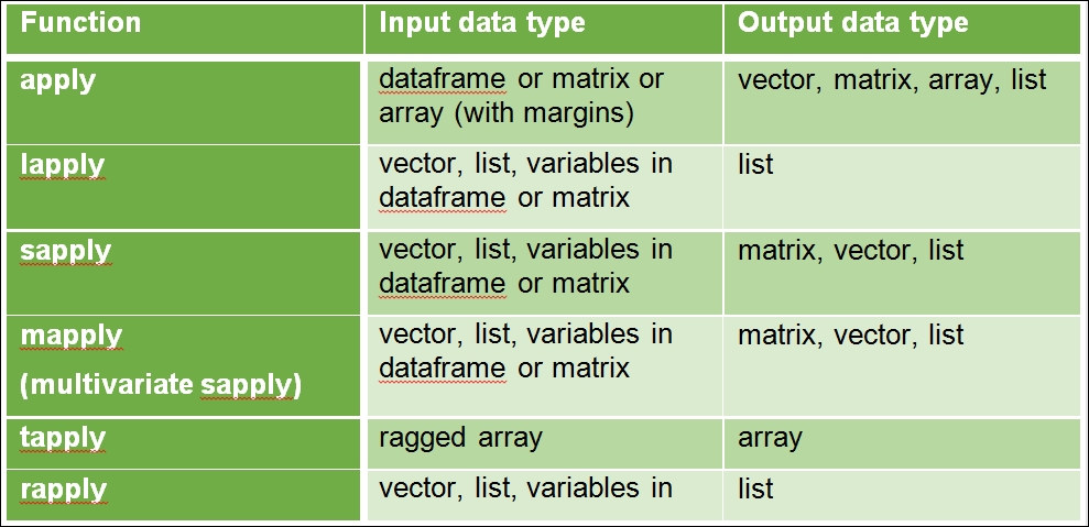
Table 1.4 Various types of functions in the apply family
Now, lets' evaluate the first class function through examples. An apply function can be applied to a dataframe, matrix, or array. Let's illustrate it using a matrix:
> x <- cbind(x1 = 7, x2 = c(7:1, 2:5))
> col.sums <- apply(x, 2, sum)
> row.sums <- apply(x, 1, sum)
The lapply is a first class function to be applied to a vector, list, or variables in a dataframe or matrix. An example of lapply is shown below:
> x <- list(x1 = 7:1, x2 = c(7:1, 2:5))
> lapply(x, mean)
The use of the sapply function for a vector input using customized function is shown below:
> V_in <- 1:100000 ## Input Vector
> V_out <- sapply(V_in,function(x) x^2) ## Output Vector
The function mapply is a multivariate sapply. The mapply function is the first input, followed by input parameters as shown below:
mapply(FUN, ..., MoreArgs = NULL, SIMPLIFY = T, USE.NAMES = T)
An example of mapply to replicated two vector can be obtained as:
> mapply(rep, 1:6, 6:1)
The function call rep function in R with input from 1 to 6 and is replicated as 6 to 1 using the second dimension of the mapply function. The tapply applies a function to each cell of the ragged array. For example, let's create a list with a multiple array:
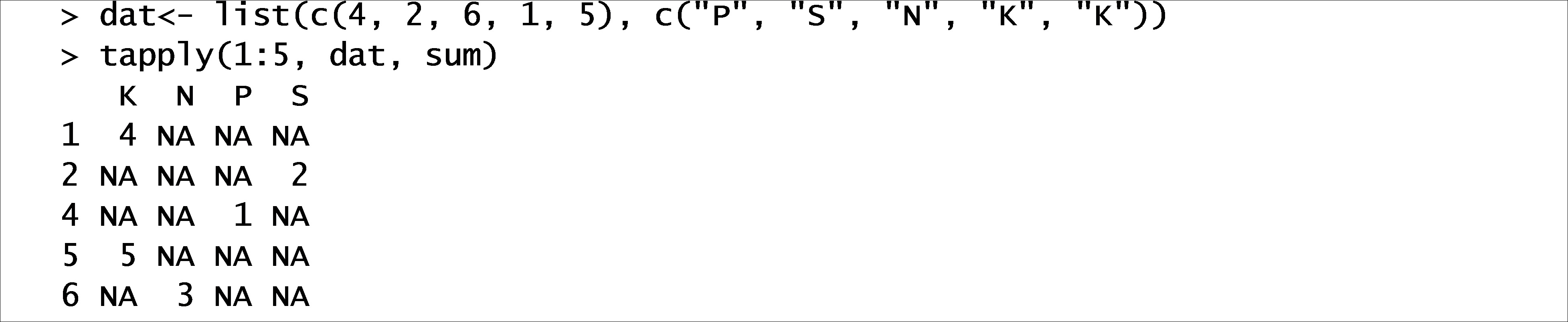
The output is a relationship between two vectors with position as a value. The function rapply is a recursive function for lapply as shown below:
> X <- list(list(a = pi, b = list(c = 1:1)), d = "a test")
> rapply(X, sqrt, classes = "numeric", how = "replace")
The function applies sqrt to all numeric classes in the list and replace it with new values.
Can you think of ways in which we can extract a few attributes (columns) and observations (rows) based on a certain condition?
Dataset - El Nino dataset from UCI KDD (https://kdd.ics.uci.edu/databases/el_nino/el_nino.html)
Filter for latitude and longitude with humidity > 88% and air temperature < 25.5 degree Celsius
10,000 iterations for evaluating each expression
Can we add multiple arguments within a function in the
applyfamily? If yes, what is the syntax for assigning multiple arguments?A general notion states that
forloops are slower than theapplyfunctions. Is it true or false? If false, what are the conditions in which the notion gets negated?Define ADT for calculating the area of any geometrical object, such as a circle, square, and so on.
Computational power has been continuously increasing in the last couple of decades, and so does the amount of data captured by different industries. To cope with data size, faster and efficient information retrieval is an eminent requirement.
In this chapter, you were introduced to ADT and data structure. ADT is used to define high-level features and operations representing different data structures, and algorithms are used to implement ADT. A data type should be atomic, traceable, accurate, and have clear and concise characteristic properties for efficiency along with unambiguity. You also learned the basics of R, including data type, conditional loops, control structure, and first class functions.
The computational time taken by an algorithm is most important objective considered while selecting data structures and algorithms. The next chapter will provide the fundamentals for the analysis of algorithms.