


 Download code from GitHub
Foundations of Haskell
In this chapter, we will cover the following recipes:
- Getting started with Haskell
- Working with data types
- Working with pure functions and user-defined data types
- Working with list functions
Introduction
We all love programs! On one side, there are surgical programming languages such as C and C++, which can solve the problem with clinical efficiency. This can be good and bad at the same time. A very experienced programmer can write a very efficient code; at the same time, it is also possible to write code that is unintelligible and very difficult to understand. On the other side, there are programs that are elegant, composable, and not only easier to understand, but also easier to reason with, such as Lisp, ML, and Haskell.
It is the second kind of programs that we will be looking at in this book. Not that efficiency is not important to us, nor does it mean that we cannot write elegant programs in C/C++. However, we will concentrate more on expressiveness, modularity, and composability of the programs. We will be interested more on the what of the program and not really on the how of the program.
Understanding the difference between what and how is very critical to understand the expressiveness, composability, and reasoning power of functional languages. Working with functional languages involves working with expressions and evaluations of expressions. The programmer builds functions consisting of expressions and composes them together to solve a problem at hand. Essentially, a functional programmer is working towards construction of a function to solve the problem that they are working on.
We will look at a program written in Haskell. The program adds two integers and returns the result of addition as follows:
    add :: Int -> Int -> Int
    add a b = a + b
Here, the add function takes two arguments, which are applied to the expression on the right-hand side. Hence, the expression add a b is equivalent to a + b. Unlike programming languages such as C/C++, add a b is not an instruction, but expressions and application of the values a and b to the expression on the right-hand side and the value of the expression. In short, one can say that add a b is bound to value of the expression a + b. When we call add 10 20, the expression is applied to the values 10 and 20, respectively. In this way, the add function is equivalent to a value that evaluates to an expression to which two values can be applied.
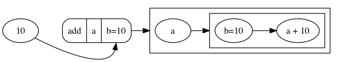
The functional program is free to evaluate the expression in multiple ways. One possible execution in a functional context is shown in the following diagram. You can see that add a b is an expression with two variables a and b as follows:
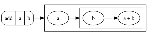
When value 10 is bound to variable b, the expression substitutes the value of b in the expression on the right-hand side:
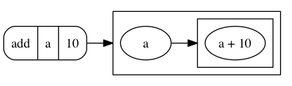
Now, the whole expression is reduced to an expression in a:
When value 20 is bound to variable a, the expression again substitutes the value of a in the expression on the right-hand side:
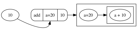
Finally, the expression is reduced to a simple expression:
Note that in the expression add a b, a and b can both be expressions. We can either evaluate the expressions before substitution, or we can substitute the expressions first and then reduce them. For example, an expression add (add 10 20) 30 can be substituted in the expression a + b as follows:
add (add 10 20) 30 = (10 + 20) + 30
Alternatively, it can be substituted by evaluating add 10 20 first and then substituting in the expression as follows:
    add (add 10 20) 30 = add (10 + 20) 30
                       = add 30 30
                       = 30 + 30
The first approach is called call by name, and the second approach is called call by value. Whichever approach we take, the value of the expression remains the same. In practice, languages such as Haskell take an intelligent approach, which is more geared towards efficiency. In Haskell, expressions are typically reduced to weak-headed normal form in which not the whole expression is evaluated, but rather a selective reduction is carried out and then is substituted in the expression.
Getting started with Haskell
In this recipe, we will work with Glasgow Haskell Compiler (GHC) and its interpreter GHCi. Then, we will write our first Haskell program and run it in the interpreter.
How to do it...
We will install Stack, a modern tool to maintain different versions of GHC and to work with different packages. Perform the following steps:
- Install Stack. Visit https://docs.haskellstack.org/en/stable/README/ and follow the instructions for your operating system.
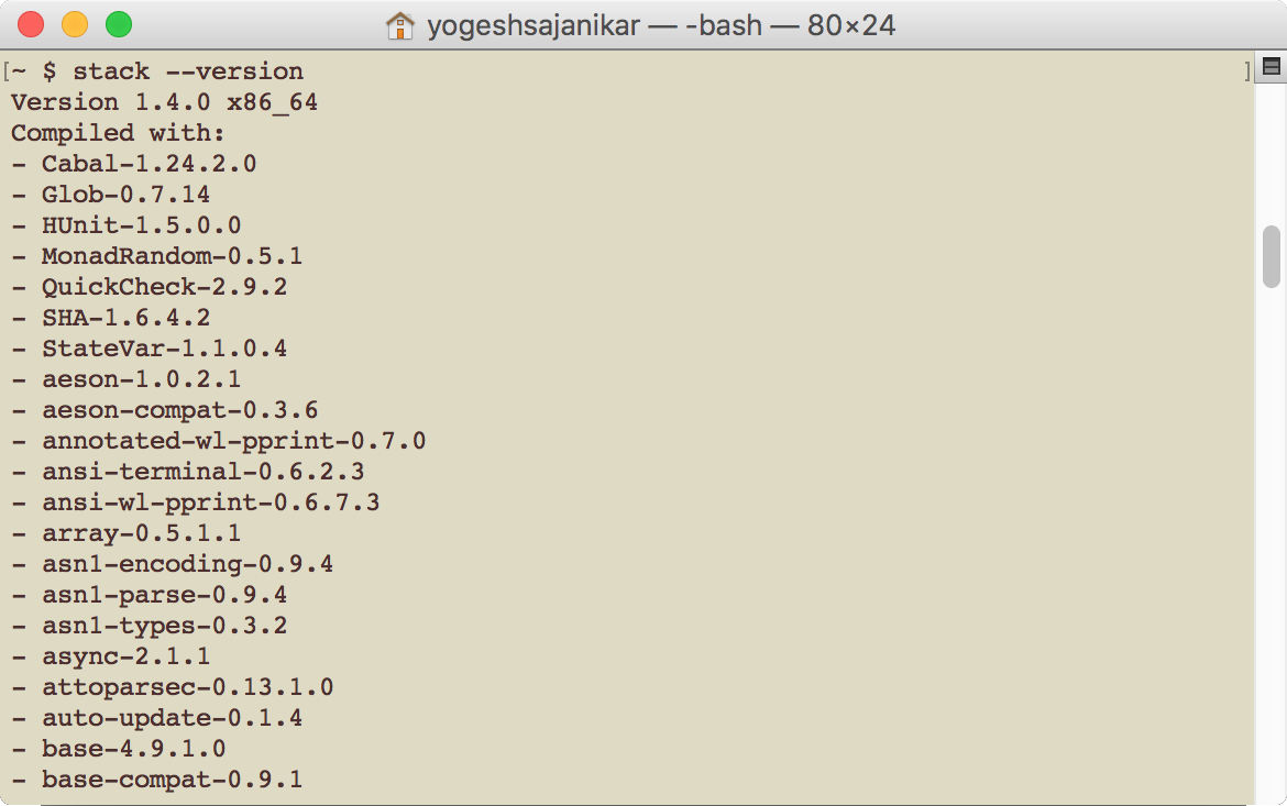
- Check that Stack works for your system by running the command stack --version at the command prompt.
Check the latest GHC version by visiting https://www.haskell.org/ghc/. Set up GHC on your box by providing the GHC version number:
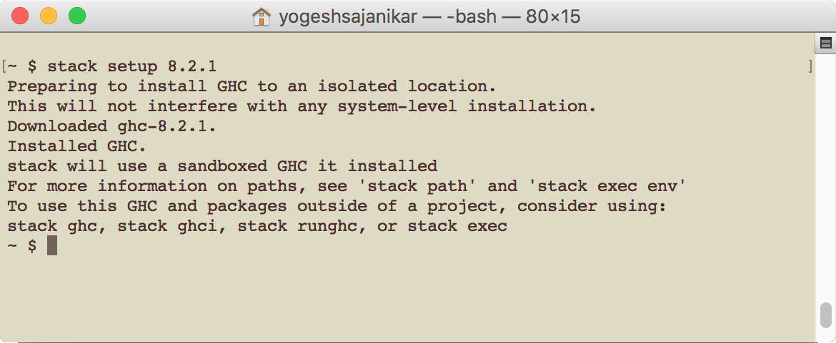
-
If you have already set up GHC on your box, then you will see the following output:
- Pick up your editor. You can set up your favorite editor to edit Haskell code. Preferable editors are Emacs, Vi, and Sublime. Once you have picked up your favorite editor, ensure that the executables for the editor remain in your path or note down the full path to the executable.
Let's create a new project, hello. Create the new project hello by running the following command in the command prompt in an empty directory:
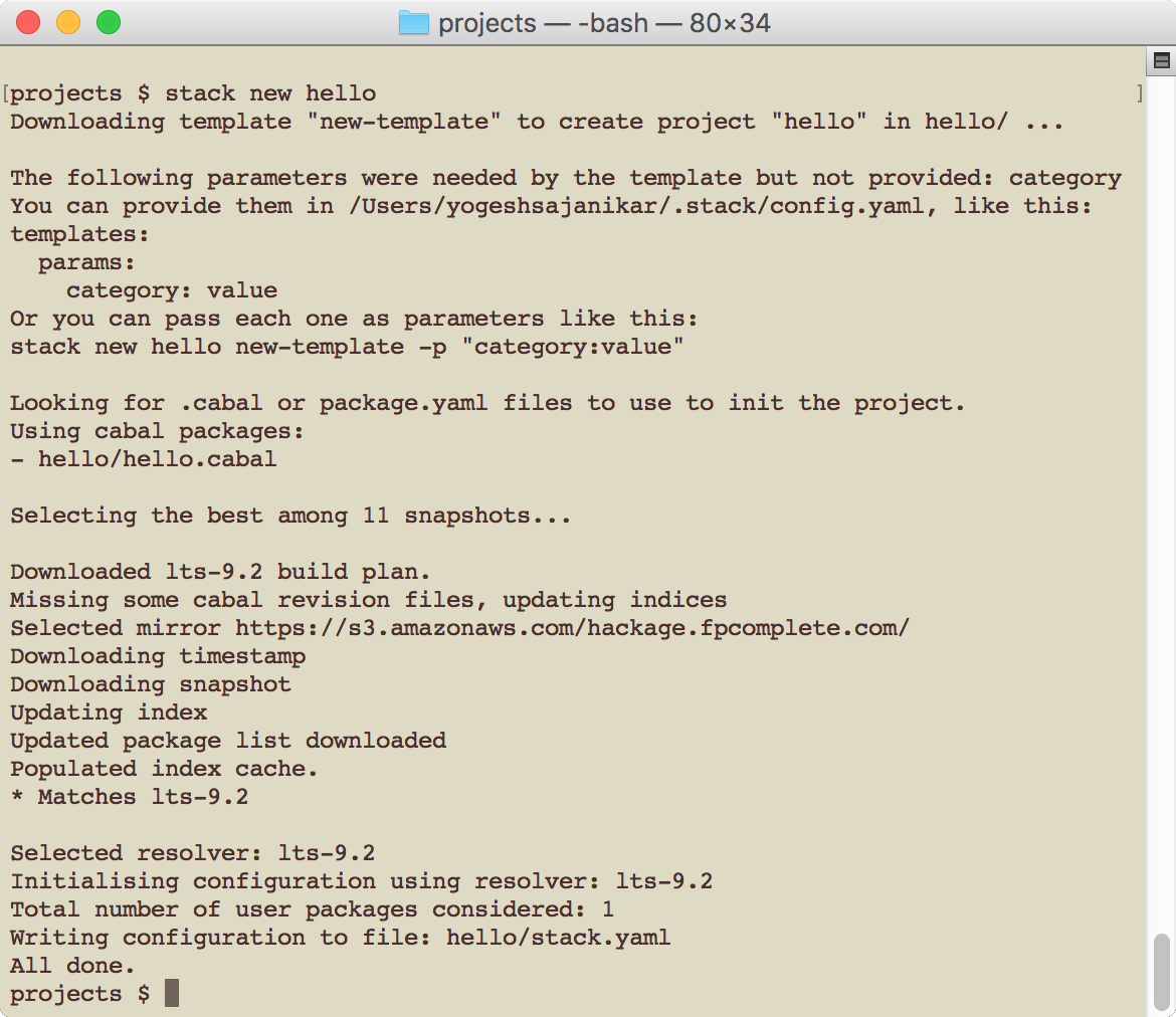
-
Change to project directory (hello) and run stack setup. When run from the new project directory, Stack automatically downloads the corresponding GHC and sets it up.
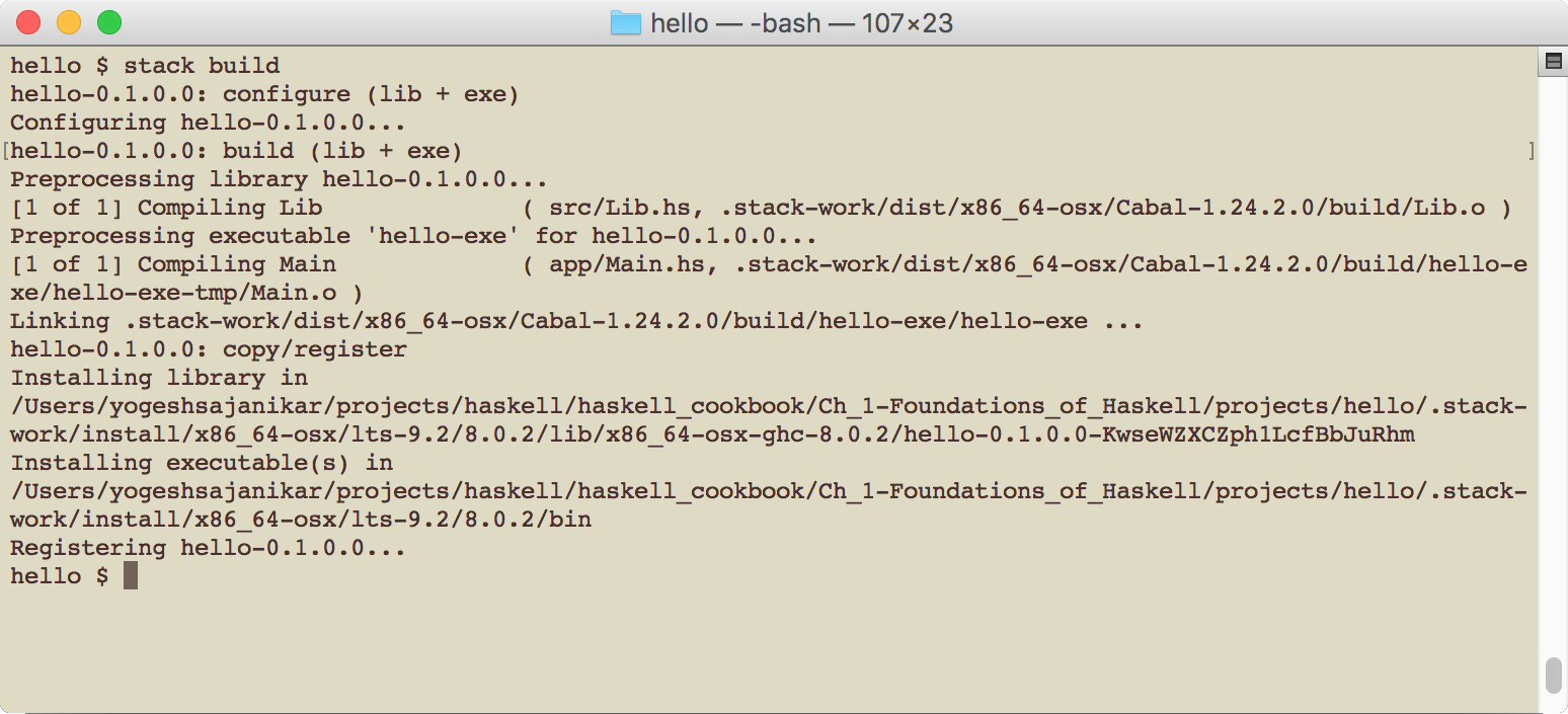
- Compile and build the project:
- You can now run the project using the following command:
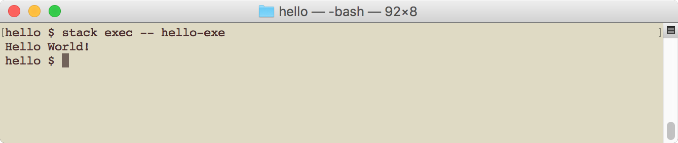
- You should see the reply someFunc printed on the console. It means that the program compilation and execution was successful.
- Inspect the hello project by opening an explorer (or file finder) and exploring the hello directory:
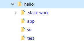
- The project contains two main directories, app and src. The library code goes into the src folder, whereas the main executable producing code goes into the app folder.
- We are interested in the app/Main.hs file.
- Now, we will set an editor. You can set the editor by defining environment variable EDITOR to point to the full path of the editor's executable.
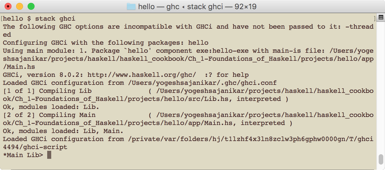
- Run the GHC interpreter by opening the command prompt and traversing to the hello project directory. Then, execute the command stack ghci. You will see the following output:
Set an editor if you haven't done so already. We are using Vi editor:
*Main Lib> :set editor gvim
- Open the Main.hs file in the editor:
*Main Lib> :edit app/Main.hs
This will open the app/Main.hs file in the window:
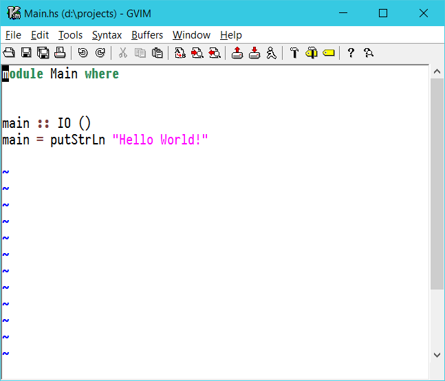
- Enter the following source in the editor:
      module Main where

      -- Single line comment!
      main :: IO ()
      main = putStrLn "Hello World!"
- Save the source file and exit. You will see that GHCi has successfully loaded the saved file:
      [2 of 2] Compiling Main
      ( d:\projects\hello\app\Main.hs, interpreted )
      Ok, modules loaded: Lib, Main.
      *Main>
- Now, you can run the main function that we have defined in the source file, and you will see the Hello World message:
        *Main> main
        Hello World!
Exit the GHCi by running :quit in the prompt.
- You can now rebuild and run the program by running the following commands:
      stack build
      stack exec -- hello-exe
You will again see the output Hello World as shown in the following screenshot:

How it works…
This recipe demonstrated the usage of Stack to create a new project, build it, set up the corresponding GHC version, build the project, and run it. The recipe also demonstrated the use of the Haskell command prompt, aka GHCi, to load and edit the file. GHCi also allows us to run the program in the command prompt.
The recipe also shows the familiar Hello World! program and how to write it. The program can be interpreted in the following way.
Dissecting Hello World
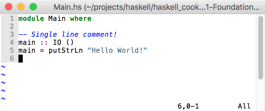
We will now look at different parts of the Main.hs program that we just created to understand the structure of a typical Haskell program. For convenience, the screenshot of the program is attached here:
The first line means that we are defining a module called Main. The source that follows where is contained in this module. In the absence of any specifications, all the functions defined in the module are exported, that is, they will be available to be used by importing the Main module.
The line number 3 (in the screenshot) that starts with -- is a comment. -- is used to represent a single-line comment. It can appear anywhere in the source code and comments on everything until the end of the line.
The next line is this:
main :: IO ()
This is a declaration of a function. :: is a keyword in Haskell, and you can read :: as has type. IO is a higher order data type as it takes a parameter (IO is a special data type called IO monad; we will see more of it at the later). () is an empty tuple and is a parameter to IO. An empty tuple in Haskell is equivalent to Unit Type. One can say that it is equivalent to void in imperative languages.
Hence, main :: IO () should be interpreted as follows:
main has a type IO ()
The next line actually defines the function:
main = putStrLn "Hello World"
It simply means that main is a function whose value is equivalent to an expression on the right-hand side, putStrLn "Hello World".
The putStrLn is a function defined in Prelude, and you can look up the type of the function by entering the following command in the prompt:
Prelude> :type putStrLn
putStrLn :: String -> IO ()
Here, putStrLn has a type String -> IO (). It means that putStrLn is a function that, when applied and when the argument is of String type, will have the resultant type IO (). Note how it matches with our type declaration of the main function.
The function declaration in the source code in Haskell is not compulsory, and the Haskell compiler can figure out the type of the function all by itself by looking at the definition of the function. You can try this by again editing the source file and removing declaration.
To edit the same file again, you can just issue the :edit command without any parameter. GHCi will open the editor with the previously opened file. To reload the file again, you can issue the :reload command and GHCi will load the file.
Now, you can verify the type of main function by issuing :t main (:t is equivalent to :type). Verify that the type of main is IO ().
There's more…
If you visit the Stack website at https://www.stackage.org/, you will notice that Stack publishes nightly packages and Long Term Support (LTS) packages. While creating a new project, Stack downloads the latest LTS package list. It is also possible to provide the name of the LTS package explicitly by providing stack new –resolver lts-9.2.
In the project directory, you will notice two files:
- <project>.yaml
- <project>.cabal
The YAML file is created by Stack to specify various things, including LTS version, external packages, and so on. The .cabal file is the main project file for the Haskell package. The cabal is the tool that Stack uses internally to build, package, and so on. However, there are several advantages of using Stack as Stack also supports pre-built packages and manages cabal well. Furthermore, Stack also supports the Docker environment.
Working with data types
In this recipe, we will work with basic data types in Haskell. We will also define our own data types.
How to do it…
- Create a new project data-types using Stack new data types. Change into the directory data-types and build the new project using stack build.
In the command prompt, run stack ghci. You will see the prompt. Enter this =:type (5 :: Int) =: command:
      *Main Lib> :type (5 :: Int)
        (5 :: Int) :: Int
:type is a GHCi command to show the type of the expression. In this case, the expression is 5. It means that the expression (5 :: Int) is Int. Now, enter this :type 5 command:
      *Main Lib> :type 5
        5 :: Num t => t
- GHCi will interpret 5 as 5 :: Num t => t, which means that Haskell identified 5 as some numerical type t. Num t => t shows that the type is t and that it has an extra qualification, Num. Num t denotes that t is an instance of a type class Num. We will see type classes later. The Num class implements functions required for numerical calculation. Note that the result of :type 5 is different from :type (5::Int).
- Now, enter :type (5 :: Double). You will see (5 :: Double) :: Double. Do the same thing with 5::Float:
      *Main Lib> :type (5 :: Double)
      (5 :: Double) :: Double
Note the difference between 5, 5::Int, 5::Float, and 5::Double. Without a qualification type (such as :: Int), Haskell interprets the type as a generic type Num t => t, that is, 5 is some type t, which is a Num t or numerical type.
Now enter following boolean types at the prompt:
      *Main Lib> :type True
      True :: Bool
      *Main Lib> :type False
      False :: Bool
True and False are valid boolean values, and their type is Bool. In fact, True and False are the only valid Bool values in Haskell. If you try 1 :: Bool, you will see an error:
      *Main Lib> 1 :: Bool

      <interactive>:9:1: error:
      * No instance for (Num Bool) arising from the literal
        ‘1’
      * In the expression: 1 :: Bool
        In an equation for ‘it’: it = 1 :: Bool
Haskell will complain that 1 is a numerical type and Bool is not a numerical type, which would somehow represent it (value 1).
- Now, type :type 'C' in the prompt. GHCi will report its type to be 'C' :: Char. Char is another data type and represents a Unicode character. A character is entered within single quotes.
- Get more information about each type. To do this, you can enter :info <type> in the prompt:
      *Main Lib> :info Bool
      data Bool = False | True
      -- Defined in ‘ghc-prim-0.5.0.0:GHC.Types’
      instance Bounded Bool -- Defined in ‘GHC.Enum’
      instance Enum Bool -- Defined in ‘GHC.Enum’
      instance Eq Bool -- Defined in ‘ghc-prim-0.5.0.0:GHC.Classes’
      instance Ord Bool -- Defined in ‘ghc-prim-0.5.0.0:GHC.Classes’
      instance Read Bool -- Defined in ‘GHC.Read’
      instance Show Bool -- Defined in ‘GHC.Show’
This will show more information about the type. For Bool, Haskell shows that it has two values False | True and that it is defined in ghc-prim-0.5.0.0:GHC.Types. Here, ghc-prim is the package name, which is followed by its version 0.5.0.0 and then Haskell tells that GHC.Types is the module in which it is defined.
How it works...
We have seen four basic types Int, Double, Char, and Float. More information about these types is given in the following table:
| Type | Description | Remarks |
| Int | Fixed precision integer type |
Range [-9223372036854775808 to 9223372036854775807] for 64-bit Int. |
| Float | Single precision (32-bit) floating point number | |
| Double | Double precision (64-bit) floating point number | |
| Char | Character | |
| Bool | Boolean values | True or False |
In previous sections of this recipe, when we ran the command :info Bool, at GHCi prompt, Haskell also showed various instances of information. It shows more about the behavior of the type. For example, instance Eq Bool means that the type Bool is an instance of some type class Eq. In Haskell, type class should be read as a type that is associated with some behavior (or function). Here, the Eq type class is used in Haskell for showing equality.
There's more…
You can get more information about type classes by exploring :info Eq. GHCi will tell you which types have instances of the Eq type class. GHCi will also tell you which are the methods defined for Eq.
Working with pure functions and user-defined data types
In this recipe, we will work with pure functions and define simple user-defined data types. We will represent a quadratic equation and its solution using user-defined data types. We will then define pure functions to find a solution to the quadratic equation.
Getting ready
- Create a new project quadratic using the following command:
stack new quadratic
Change into the project folder.
- Delete src/Lib.hs and create a new file src/Quadratic.hs to represent the quadratic equation and its solution.
- Open the quadratic.cabal file, and in the section library, replace Lib by Quadratic in the tag exposed-modules:
      library
        hs-source-dirs:      src
        exposed-modules:     Quadratic
        build-depends:       base >= 4.7 && < 5
        default-language:    Haskell2010
How to do it...
- Open Quadratic.hs and add a module definition to it:
module Quadratic where
- Import the standard module Data.Complex to help us represent a complex solution to the quadratic equation.
- Define the data type to represent the quadratic equation:
      data Quadratic = Quadratic { a :: Double, b :: Double,
        c :: Double }
        deriving Show
This represents the quadratic equation of the form a∗x2+b∗x+c=0a∗x2+b∗x+c=0. a, b, and c represent the corresponding constants in the equation.
- Define the data type for representing the root:
type RootT = Complex Double
This represents that the complex data type parameterized by Double. RootT is synonymous to type Complex Double (similar to typedef in C/C++).
- A quadratic equation has two roots, and hence we can represent both the roots as follows:
      import Data.Complex
        type RootT = Complex Double
        data Roots = Roots RootT RootT deriving Show
- Implement the solution. We will take a top-down approach to create a solution. We will define a top-level function where we will implement a function assuming lower level details:
roots :: Quadratic -> Roots
This shows that the roots function takes one argument of type Quadratic, and returns Roots.
- Implement three cases mentioned next:
      -- | Calculates roots of a polynomial and return set of roots
      roots :: Quadratic -> Roots

      -- Trivial, all constants are zero, error roots are not defined
      roots (Quadratic 0 0 _) = error "Not a quadratic polynomial"

      -- Is a polynomial of degree 1, x = -c / b
      roots (Quadratic 0.0 b c) = let root = ( (-c) / b :+ 0)
                            in Roots root root

      -- b^2 - 4ac = 0
      roots (Quadratic a b c) =
      let discriminant = b * b - 4 * a * c
      in rootsInternal (Quadratic a b c) discriminant
We have referred to the rootsInternal function, which should handle case A, B, and C for the case III.
- Implement the rootsInternal function to find all roots of the quadratic equation:
      rootsInternal :: Quadratic -> Double -> Roots
      -- Discriminant is zero, roots are real
      rootsInternal q d | d == 0 = let r = (-(b q) / 2.0 / (a q))
                                 root = r :+ 0
                             in Roots root root

      -- Discriminant is negative, roots are complex
      rootsInternal q d | d < 0 = Roots (realpart :+ complexpart)
     (realpart :+ (-complexpart))
      where plusd = -d
        twoa = 2.0 * (a q)
        complexpart = (sqrt plusd) / twoa
        realpart = - (b q) / twoa

      -- discriminant is positive, all roots are real
      rootsInternal q d = Roots (root1 :+ 0) (root2 :+ 0)
      where plusd = -d
        twoa = 2.0 * (a q)
        dpart = (sqrt plusd) / twoa
        prefix = - (b q) / twoa
        root1 = prefix + dpart
        root2 = prefix - dpart
Open src/Main.hs. We will use the Quadratic module here to solve a couple of quadratic equations. Add the following lines of code in Main.hs:
      module Main where

      import Quadratic
      import Data.Complex

      main :: IO ()
      main = do
        putStrLn $ show $ roots (Quadratic 0 1 2)
        putStrLn $ show $ roots (Quadratic 1 3 4)
        putStrLn $ show $ roots (Quadratic 1 3 4)
        putStrLn $ show $ roots (Quadratic 1 4 4)
        putStrLn $ show $ roots (Quadratic 1 0 4)
- Execute the application by building the project using stack build and then executing with stack exec – quadratic-exe in the command prompt. You will see the following output:
      Roots ((-2.0) :+ 0.0) ((-2.0) :+ 0.0)
      Roots ((-1.5) :+ 1.3228756555322954) ((-1.5) :+
      (-1.3228756555322954))
      Roots ((-1.5) :+ 1.3228756555322954) ((-1.5) :+
      (-1.3228756555322954))
      Roots ((-2.0) :+ 0.0) ((-2.0) :+ 0.0)
      Roots ((-0.0) :+ 2.0) ((-0.0) :+ (-2.0))
How it works...
A quadratic equation is represented by ax^2 + bx + c = 0. There are three possible cases that we have to handle:
| Case | Condition | Root 1 | Root 2 | Remarks |
| I | a = 0 and b = 0 | ERROR | ERROR | |
| II | a = 0 | x = -c/b | Not applicable | Linear equation |
| III | a and b are non-zero, delta = b2 - 4ac | |||
| III-A | delta = 0 | -b/(2a) | -b/(2a) | Perfect square |
| III-B | delta > 0 | (-b+sqrt(delta))/(2a) | (-b-sqrt(delta))/(2a) | Real roots |
| III-C | delta < 0 | (-b+sqrt(delta))/(2a) | (-b-sqrt(delta))/(2a) | Complex roots |
We will define a module at the top of the file with the Quadratic module where the name of the module matches file name, and it starts with a capital letter. The Quadratic module is followed by the definition of module (data types and functions therein). This exports all data types and functions to be used by importing the module.
We will import the standard Data.Complex module. The modules can be nested. Many useful and important modules are defined in the base package. Every module automatically includes a predefined module called Prelude. The Prelude exports many standard modules and useful functions. For more information on base modules, refer to https://hackage.haskell.org/package/base.
The user-defined data is defined by the keyword data followed by the name of the data type. The data type name always start with a capital letter (for example, data Quadratic).
Here, we will define Quadratic as follows:
    data Quadratic = Quadratic { a :: Double, b ::
      Double, c :: Double  }
      deriving Show
There are several things to notice here:
- The name on the left-hand side, Quadratic, is called type constructor. It can take one or more data types. In this case, we have none.
- The name Quadratic on the right-hand is called data constructor. It is used to create the value of the type defined on the left-hand side.
- {a :: Double, b :: Double, c :: Double } is called the record syntax for defining fields. a, b and c are fields, each of type Double.
- Each field is a function in itself that takes data type as the first argument and returns the value of the field. In the preceding case, a will have the function type Quadratic -> Double, which means a will take the value of type Quadratic as the first argument and return the field a of type Double.
- The definition of data type is followed by deriving Show. Show is a standard type class in Haskell and is used to convert the value to String. In this case, Haskell can automatically generate the definition of Show. However, it is also possible to write our own definition. Usually, the definition generated by Haskell is sufficient.
We will define root as type Complex Double. The data type Complex is defined in the module Data.Complex, and its type constructor is parameterized by a type parameter a. In fact, the Complex type is defined as follows:
data Complex a = a :+ a
There are several things to notice here. First, the type constructor of Complex takes an argument a. This is called type argument, as the Complex type can be constructed with any type a.
The second thing to note is how the data constructor is defined. The data constructor's name is not alphanumeric, and it is allowed.
Note that the data constructor takes two parameters. In such a case, data constructor can be used with infix notation. That is, you can use the constructor in between two arguments.
The third thing to note is that the type parameter used in the type constructor can be used as a type while defining the data constructor.
Since our quadratic equation is defined in terms of Double, the complex root will always have a type Complex Double. Hence, we will define a type synonym using the following command:
type RootT = Complex Double
We will define two roots of the equation using the following command:
data Roots = Roots RootT RootT deriving Show
Here, we have not used the record syntax, but just decided to create two anonymous fields of type RootT with data constructor Roots.
The roots function is defined as follows:
roots :: Quadratic -> Roots
It can be interpreted as the roots function has a type Quadratic -> Roots, which is a function that takes a value of type Quadratic and returns a value of type Roots:
- Pattern matching: We can write values by exploding data constructor in the function arguments. Haskell matches these values and then calls the definition on the right-hand side. In Haskell, we can separate the function definition using such matching. Here, we will use pattern matching to separate cases I, II, and III, defined in the preceding section. The case I can be matched with value (Quadratic 0 0 _) where the first two zeros match fields a and b, respectively. The last field is specified by _, which means that we do not care about this value, and it should not be evaluated.
- Raising an error: For the first case, we flag an error by using function error. The function error takes a string and has a signature (error :: String -> a) which means that it takes a String and returns value of any type a. Here, it raises an exception.
- let .. in clause: In the case II as mentioned in the preceding section, we use let ... in clause.
        let root = ( (-c) / b :+ 0)
        in Roots root root
Here, the let clause is used to bind identifiers (which always start with a lowercase letter; so do function names). The let clause is followed by the in clause. The in clause has the expression that is the value of the let…in clause. The in expression can use identifiers defined in let. Furthermore, let can bind multiple identifiers and can define functions as well.
We defined rootsInternal as a function to actually calculate the roots of a quadratic equation. The rootsInternal function uses pattern guards. The pattern guards are explained as follows:
- Pattern guards: The pattern guards are conditions that are defined after a vertical bar | after the function arguments. The pattern guard defines a condition. If the condition is satisfied, then the expression on the right-hand side is evaluated:
rootsInternal q d | d == 0 = ...
In the preceding definition, d == 0 defines the pattern guard. If this condition is satisfied, then the function definition is bound to the expression on the right-hand side.
- where clause: The rootsInternal function also uses the where clause. This is another form of the let…in clause:
        let <bindings>
        in <expression>
It translates to the following lines of code:
        <expression>
        where
        <bindings>
In Main.hs, we will import the Quadratic module and use the functions and data type defined in it. We will use the do syntax, which is used in conjunction with the IO type, for printing to the console, reading from the console, and, in general, for interfacing with the outside world.
The putStrLn function prints the string to the console. The function converts a value to a string. This is enabled because of auto-definition due to deriving Show.
We will use a data constructor to create values of Quadratic. We can simply specify all the fields in the order such as, Quadratic 1 3 4, where a = 1, b = 3, and c = 4. We can also specify the value of Quadratic using record syntax, such as Quadratic { a = 10, b = 30, c = 5 }.
Things are normally put in brackets, as shown here:
putStrLn (show (roots (Quadratic 0 1 2)))
However, in this case, we will use a special function $, which simplifies the application of brackets and allows us to apply arguments to the function from right to left as shown:
putStrLn $ show $ roots (Quadratic 0 1 2)
Source formatting
You must have also noticed how the Haskell source code is formatted. The blocks are indented by white spaces. There is no hard and fast rule for indenting; however, it must be noted that there has to be a significant white space indent for a source code block, such as the let clause or the where clause. A simple guideline is that any block should be indented in such a way that it is left aligned and increases the readability of the code. A good Haskell source is easy to read.
Working with list functions
In this recipe, we will work with the list data type in Haskell. The list function is one of the most widely used data types in Haskell.
Getting ready
Use Stack to create a new project, list functions, and change into the project directory. Build the project with stack build.
Remove the contents of src/Lib.hs and add the module heading:
module Lib where
How to do it...
- Create an empty list:
emptyList = []
- Prepend an element to the list:
prepend = 10 : []
- Create a list of five integers:
list5 = 1 : 2 : 3 : 4 : 5 : []
- Create a list of integers from 1 to 10:
list10 = [1..10]
- Create an infinite list:
infiniteList = [1..]
- This is the head of a list:
getHead = head [1..10]
- This is the tail of a list:
getTail = tail [1..10]
- This is all but the last element:
allbutlast = init [1..10]
- Take 10 elements:
take10 = take 10 [1..]
- Drop 10 elements:
drop10 = drop 10 [1..20]
- Get nth element:
get1331th = [1..] !! 1331
- Check if a value is the element of the list.
is10element = elem 10 [1..10]
- Do pattern matching on the list. Here we check whether the list is empty or not:
        isEmpty [] = True
        isEmpty _ = False
- Do more pattern matching. Here we do pattern matching on elements present in the list.
        isSize2 (x:y:[]) = True
        isSize2 _ = False
- Concatenate two lists:
cat2 = [1..10] ++ [11..20]
- String is actually a list. Check this by creating a list of characters:
a2z = ['a'..'z']
- Since string is a list, we can use all list functions on string. Here we get the first character of a string:
strHead = head "abc"
- Zip two lists:
zip2 = zip ['a'..'z'] [1.. ]
- Open app/Main.hs and use the preceding functions from the list, and also print values:
        module Main where

        import Lib

        main :: IO ()
        main = do
          putStrLn $ show $ (emptyList :: [Int])
          putStrLn $ show $ prepend
          putStrLn $ show $ list5
          putStrLn $ show $ list10
          putStrLn $ show $ getHead
          putStrLn $ show $ getTail
          putStrLn $ show $ allbutlast
          putStrLn $ show $ take10
          putStrLn $ show $ drop10
          putStrLn $ show $ get1331th
          putStrLn $ show $ is10element
          putStrLn $ show $ isEmpty [10]
          putStrLn $ show $ isSize2 []
          putStrLn $ show $ cat2
          putStrLn $ show $ a2z
          putStrLn $ show $ strHead
- Build the project using stack build and run it using stack run list-functions-exe. Note that Main does not use the infiniteList snippets and does not print them.
How it works...
List is defined as follows:
    data [] a = []       -- Empty list or
       | a : [a]  -- An item prepended to a list, is also a list
There are two data constructors. The first data [] constructor shows an empty list, and a list with no elements is a valid list. The second data constructor tells us that an item prepended to a list is also a list.
Also, notice that the type constructor is parameterized by a type parameter a. It means that the list can be constructed with any type a.
List creation
The first three snippets in the previous section are created using list's data constructors. The third example shows recursive application of the second constructor.
Enumerated list
The fourth and fifth snippets show how to create a list from enumerated values. Enumerated values are those that implement type class Enum and are implemented by ordered types such as Int, Double, Float, Char, and so on. The enumerated type allows us to specify a range using '..' (for example, 1..10, which means numerals 1 to 10, including 10). It is also possible to drop the to value. For example, 1.. will create an infinite list. It is also possible to specify an increment by specifying consecutive values. For example, 1,3,..10 will expand to 1,3,5,7,9 (note that the last value 10 is not part of it as it does not belong to the sequence).
Head and tail of a list
From the definition of a list, any element, when prepended to a list, is also a list. For example, 1:[2,3] is also a list. Here, 1 is called the head of the list, and 2 is called the tail of the list.
The functions head and tail return head and tail, respectively, of the list. The snippets 6 and 7 show an example of head and tail. Head has a signature - head :: [a] -> a and tail has a signature :: [a] -> [a] .
Operations on a list
Once we have a list, we can do various operations, such as the following ones:
- init :: [a] -> [a]: Take all but the last element of the list. This is shown in snippet 8.
- take :: Int -> [a] -> [a]: Take, at the most, the first n elements of the list (shown as the Int argument). If the list has less than n elements, then it will consume the entire list. This is shown in snippet 9.
In snippet 9, we worked on an infinite list and took only the first 10 elements. This works in Haskell, because in Haskell, nothing is evaluated until computation needs a value. Hence, even if we have an infinite list, when we take the first 10 elements, only 10 elements of the list are evaluated. Such things are not possible in strict languages. Haskell is not a strict language.
- drop :: Int -> [a] -> [a]: Similar to take, but the drop function drops the first n elements. It will drop the whole list if the list has less than n elements. If we operate on an infinite list, then we will get an infinite list back. Snippet 10 shows an example of drop.
Indexed access
The function names in Haskell do not necessarily start with alphabets. Haskell allows us to use a combination of other characters as well. Many collections, including list, define !! as an indexing function. Snippet 11 uses this.
The function !! takes a list and an index n, and returns the nth element, starting 0. The signature of !! is (!!) :: Int -> [a] -> a.
It is important to note that an access to an indexed element in the list is not random. It is sequential and is directly proportional to the index value. Hence, care should be taken to use this function.
Checking whether an element is present
The elem function checks whether a given element is present in the list. The elem function must be able to equate itself with another of its own type. This is done by implementing type Eq class, which allows checking whether two values of a type are equal or not.
Pattern matching on list
Once we know that a list has two data constructors, we can use them in the function argument for pattern matching. Hence, we can use [] for empty list matching, and we can use x:y:[] to match two elements followed by an empty list.
In the snippet 13, we used an empty list pattern for checking whether a list is empty or not.
In the snippet 14, we used x:y:[] to check whether the list has length 2 or not. This might not be a very good thing if we want to check the larger size. There, we might use the length function to get the size of the list. However, be aware of the fact that the length function is not a constant time function, but proportional to the size of the list.
List concatenation
It is possible to concatenate two lists by using the ++ function. The running time of this function is directly proportional to the size of the first list.
Strings are lists
It is important to note that the type String in Haskell is implemented as a list of Char:
type String = [Char]
Hence, all list operations are valid string operations as well. The snippets 17 and 18 show this by applying list functions on String. Since list is not a random access collection and operations such as concatenation are not constant time operations, strings in Haskell are not very efficient. There are libraries such as text that implement strings in a very efficient way.
There's more…
The preceding list of operations on Haskell list is not exhaustive. You can refer to the Data.List module in the base package (which is installed as a part of GHC). It provides documentation to all the functions that operate on list.