


 Download code from GitHub
Chapter 1: Benchmarking and Profiling
Recognizing the slow parts of your program is the single most important task when it comes to speeding up your code. In most cases, the code that causes the application to slow down is a very small fraction of the program. By identifying these critical sections, you can focus on the parts that need the most improvement without wasting time in micro-optimization.
Profiling is a technique that allows us to pinpoint the most resource-intensive parts of an application. A profiler is a program that runs an application and monitors how long each function takes to execute, thus detecting the functions on which your application spends most of its time.
Python provides several tools to help us find these bottlenecks and measure important performance metrics. In this chapter, we will learn how to use the standard cProfile module and the line_profiler third-party package. We will also learn how to profile the memory consumption of an application through the memory_profiler tool. Another useful tool that we will cover is KCachegrind, which can be used to graphically display the data produced by various profilers.
Finally, benchmarks are small scripts used to assess the total execution time of your application. We will learn how to write benchmarks and use them to accurately time your programs.
The topics we will cover in this chapter are listed here:
- Designing your application
- Writing tests and benchmarks
- Writing better tests and benchmarks with
pytest-benchmark - Finding bottlenecks with
cProfile - Optimizing our code
- Using the
dismodule - Profiling memory usage with
memory_profiler
By the end of the chapter, you will have gained a solid understanding of how to optimize a Python program and will be armed with practical tools that facilitate the optimization process.
Technical requirements
To follow the content of this chapter, you should have a basic understanding of Python programming and be familiar with core concepts such as variables, classes, and functions. You should also be comfortable with working with the command line to run Python programs. Finally, the code for this chapter can be found in the following GitHub repository: https://github.com/PacktPublishing/Advanced-Python-Programming-Second-Edition/tree/main/Chapter01.
Designing your application
In the early development stages, the design of a program can change quickly and may require large rewrites and reorganizations of the code base. By testing different prototypes without the burden of optimization, you are free to devote your time and energy to ensure that the program produces correct results and that the design is flexible. After all, who needs an application that runs fast but gives the wrong answer?
The mantras that you should remember when optimizing your code are outlined here:
- Make it run: We have to get the software in a working state and ensure that it produces the correct results. This exploratory phase serves to better understand the application and to spot major design issues in the early stages.
- Make it right: We want to ensure that the design of the program is solid. Refactoring should be done before attempting any performance optimization. This really helps separate the application into independent and cohesive units that are easy to maintain.
- Make it fast: Once our program is working and well structured, we can focus on performance optimization. We may also want to optimize memory usage if that constitutes an issue.
In this section, we will write and profile a particle simulator test application. A simulator is a program that considers some particles and simulates their movement over time according to a set of laws that we impose. These particles can be abstract entities or correspond to physical objects—for example, billiard balls moving on a table, molecules in a gas, stars moving through space, smoke particles, fluids in a chamber, and so on.
Building a particle simulator
Computer simulations are useful in fields such as physics, chemistry, astronomy, and many other disciplines. The applications used to simulate systems are particularly performance-intensive, and scientists and engineers spend an inordinate amount of time optimizing their code. In order to study realistic systems, it is often necessary to simulate a very high number of bodies, and every small increase in performance counts.
In our first example, we will simulate a system containing particles that constantly rotate around a central point at various speeds, just like the hands of a clock.
The necessary information to run our simulation will be the starting positions of the particles, the speed, and the rotation direction. From these elements, we have to calculate the position of the particle in the next instant of time. An example system is shown in the following diagram. The origin of the system is the (0, 0) point, the position is indicated by the x, y vector, and the velocity is indicated by the vx, vy vector:
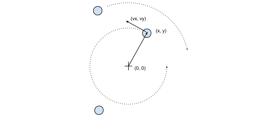
Figure 1.1 – An example of a particle system
The basic feature of a circular motion is that the particles always move perpendicular to the direction connecting the particle and the center. To move the particle, we simply change the position by taking a series of very small steps (which correspond to advancing the system for a small interval of time) in the direction of motion, as shown in the following diagram:

Figure 1.2 – Movement of a particle
We will start by designing the application in an object-oriented (OO) way. According to our requirements, it is natural to have a generic Particle class that stores the particle positions, x and y, and their angular velocity, ang_vel, as illustrated in the following code snippet:
    class Particle:
        def __init__(self, x, y, ang_vel):
            self.x = x
            self.y = y
            self.ang_vel = ang_vel
Note that we accept positive and negative numbers for all the parameters (the sign of ang_vel will simply determine the direction of rotation).
Another class, called ParticleSimulator, will encapsulate the laws of motion and will be responsible for changing the positions of the particles over time. The __init__ method will store a list of Particle instances, and the evolve method will change the particle positions according to our laws. The code is illustrated in the following snippet:
class ParticleSimulator:
    def __init__(self, particles):
        self.particles = particles
We want the particles to rotate around the position corresponding to the x=0 and y=0 coordinates, at a constant speed. The direction of the particles will always be perpendicular to the direction from the center (refer to Figure 1.1 in this chapter). To find the direction of the movement along the x and y axes (corresponding to the Python v_x and v_y variables), it is sufficient to use these formulae:
    v_x = -y / (x**2 + y**2)**0.5
    v_y = x / (x**2 + y**2)**0.5
If we let one of our particles move, after a certain time t, it will reach another position following a circular path. We can approximate a circular trajectory by dividing the time interval, t, into tiny time steps, dt, where the particle moves in a straight line tangentially to the circle. (Note that higher-order curves could be used rather than straight lines for better accuracy, but we will stick with lines as the simplest approximation.) The final result is just an approximation of a circular motion.
In order to avoid a strong divergence, such as the one illustrated in the following diagram, it is necessary to take very small time steps:
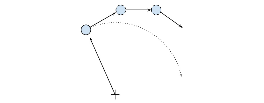
Figure 1.3 – Undesired divergence in particle motion due to large time steps
In a more schematic way, we have to carry out the following steps to calculate the particle position at time t:
- Calculate the direction of motion (
v_xandv_y). - Calculate the displacement (
d_xandd_y), which is the product of the time step, angular velocity, and direction of motion. - Repeat Steps 1 and 2 enough times to cover the total time t.
The following code snippet shows the full ParticleSimulator implementation:
    class ParticleSimulator:
        def __init__(self, particles):
            self.particles = particles
        def evolve(self, dt):
            timestep = 0.00001
            nsteps = int(dt/timestep)

            for i in range(nsteps):
                for p in self.particles:
                    # 1. calculate the direction
                    norm = (p.x**2 + p.y**2)**0.5
                    v_x = -p.y/norm
                    v_y = p.x/norm
                    # 2. calculate the displacement
                    d_x = timestep * p.ang_vel * v_x
                    d_y = timestep * p.ang_vel * v_y
                    p.x += d_x
                    p.y += d_y
                    # 3. repeat for all the time steps
And with that, we have finished building the foundation of our particle simulator. Next, we will see it in action by visualizing the simulated particles.
Visualizing the simulation
We can use the matplotlib library here to visualize our particles. This library is not included in the Python standard library, but it can be easily installed using the pip install matplotlib command.
Alternatively, you can use the Anaconda Python distribution (https://store.continuum.io/cshop/anaconda/), which includes matplotlib and most of the other third-party packages used in this book. Anaconda is free and is available for Linux, Windows, and Mac.
To make an interactive visualization, we will use the matplotlib.pyplot.plot function to display the particles as points and the matplotlib.animation.FuncAnimation class to animate the evolution of the particles over time.
The visualize function takes a ParticleSimulator particle instance as an argument and displays the trajectory in an animated plot. The steps necessary to display the particle trajectory using the matplotlib tools are outlined here:
- Set up the axes and use the
plotfunction to display the particles. Theplotfunction takes a list of x and y coordinates. - Write an initialization function,
init, and a function,animate, that updates the x and y coordinates using theline.set_datamethod. Note that ininit, we need to return the line data in the form ofline, due to syntactic reasons. - Create a
FuncAnimationinstance by passing theinitandanimatefunctions and theintervalparameters, which specify the update interval, andblit, which improves the update rate of the image. - Run the animation with
plt.show(), as illustrated in the following code snippet:from matplotlib import pyplot as plt from matplotlib import animation def visualize(simulator): X = [p.x for p in simulator.particles] Y = [p.y for p in simulator.particles] fig = plt.figure() ax = plt.subplot(111, aspect='equal') line, = ax.plot(X, Y, 'ro') # Axis limits plt.xlim(-1, 1) plt.ylim(-1, 1) # It will be run when the animation starts def init(): line.set_data([], []) return line, # The comma is important! def animate(i): # We let the particle evolve for 0.01 time units simulator.evolve(0.01) X = [p.x for p in simulator.particles] Y = [p.y for p in simulator.particles] line.set_data(X, Y) return line, # Call the animate function each 10 ms anim = animation.FuncAnimation(fig, animate,init_func=init,blit=True, interval=10) plt.show()
To test this code, we define a small function, test_visualize, that animates a system of three particles rotating in different directions. Note in the following code snippet that the third particle completes a round three times faster than the others:
    def test_visualize():
        particles = [
                     Particle(0.3, 0.5, 1),
                     Particle(0.0, -0.5, -1),
                     Particle(-0.1, -0.4, 3)
        ]
        simulator = ParticleSimulator(particles)
        visualize(simulator)
    if __name__ == '__main__':
        test_visualize()
The test_visualize function is helpful to graphically understand the system time evolution. Simply close the animation window when you'd like to terminate the program. With this program in hand, in the following section, we will write more test functions to properly verify program correctness and measure performance.
Writing tests and benchmarks
Now that we have a working simulator, we can start measuring our performance and tune up our code so that the simulator can handle as many particles as possible. As a first step, we will write a test and a benchmark.
We need a test that checks whether the results produced by the simulation are correct or not. Optimizing a program commonly requires employing multiple strategies; as we rewrite our code multiple times, bugs may easily be introduced. A solid test suite ensures that the implementation is correct at every iteration so that we are free to go wild and try different things with the confidence that, if the test suite passes, the code will still work as expected. More specifically, what we are implementing here are called unit tests, which aim to verify the intended logic of the program regardless of the implementation details, which may change during optimization.
Our test will take three particles, simulate them for 0.1 time units, and compare the results with those from a reference implementation. A good way to organize your tests is using a separate function for each different aspect (or unit) of your application. Since our current functionality is included in the evolve method, our function will be named test_evolve. The following code snippet shows the test_evolve implementation. Note that, in this case, we compare floating-point numbers up to a certain precision through the fequal function:
    def test_evolve():
        particles = [Particle( 0.3,  0.5, +1),
                     Particle( 0.0, -0.5, -1),
                     Particle(-0.1, -0.4, +3)
            ]
        simulator = ParticleSimulator(particles)
        simulator.evolve(0.1)
        p0, p1, p2 = particles
        def fequal(a, b, eps=1e-5):
            return abs(a - b) < eps
        assert fequal(p0.x, 0.210269)
        assert fequal(p0.y, 0.543863)
        assert fequal(p1.x, -0.099334)
        assert fequal(p1.y, -0.490034)
        assert fequal(p2.x,  0.191358)
        assert fequal(p2.y, -0.365227)
    if __name__ == '__main__':
        test_evolve()
The assert statements will raise an error if the included conditions are not satisfied. Upon running the test_evolve function, if you notice no error or output printed out, that means all the conditions are met.
A test ensures the correctness of our functionality but gives little information about its running time. A benchmark is a simple and representative use case that can be run to assess the running time of an application. Benchmarks are very useful to keep score of how fast our program is with each new version that we implement.
We can write a representative benchmark by instantiating a thousand Particle objects with random coordinates and angular velocity and feeding them to a ParticleSimulator class. We then let the system evolve for 0.1 time units. The code is illustrated in the following snippet:
    from random import uniform
    def benchmark():
        particles = [
          Particle(uniform(-1.0, 1.0), uniform(-1.0, 1.0),
            uniform(-1.0, 1.0))
          for i in range(1000)]
        simulator = ParticleSimulator(particles)
        simulator.evolve(0.1)
    if __name__ == '__main__':
        benchmark()
With the benchmark program implemented, we now need to run it and keep track of the time needed for the benchmark to complete execution, which we will see next. (Note that when you run these tests and benchmarks on your own system, you are likely to see different numbers listed in the text, which is completely normal and dependent on your system configurations and Python version.)
Timing your benchmark
A very simple way to time a benchmark is through the Unix time command. Using the time command, as follows, you can easily measure the execution time of an arbitrary process:
    $ time python simul.py
real    0m1.051s
user    0m1.022s
sys     0m0.028s
The time command is not available for Windows. To install Unix tools such as time on Windows, you can use the cygwin shell, downloadable from the official website (http://www.cygwin.com/). Alternatively, you can use similar PowerShell commands, such as Measure-Command (https://msdn.microsoft.com/en-us/powershell/reference/5.1/microsoft.powershell.utility/measure-command), to measure execution time.
By default, time displays three metrics, as outlined here:
real: The actual time spent running the process from start to finish, as if it were measured by a human with a stopwatch.user: The cumulative time spent by all the central processing units (CPUs) during the computation.sys: The cumulative time spent by all the CPUs during system-related tasks, such as memory allocation.Note
Sometimes,
userandsysmight be greater thanreal, as multiple processors may work in parallel.
time also offers richer formatting options. For an overview, you can explore its manual (using the man time command). If you want a summary of all the metrics available, you can use the -v option.
The Unix time command is one of the simplest and most direct ways to benchmark a program. For an accurate measurement, the benchmark should be designed to have a long enough execution time (in the order of seconds) so that the setup and teardown of the process are small compared to the execution time of the application. The user metric is suitable as a monitor for the CPU performance, while the real metric also includes the time spent on other processes while waiting for input/output (I/O) operations.
Another convenient way to time Python scripts is the timeit module. This module runs a snippet of code in a loop for n times and measures the total execution time. Then, it repeats the same operation r times (by default, the value of r is 3) and records the time of the best run. Due to this timing scheme, timeit is an appropriate tool to accurately time small statements in isolation.
The timeit module can be used as a Python package, from the command line or from IPython.
IPython is a Python shell design that improves the interactivity of the Python interpreter. It boosts tab completion and many utilities to time, profile, and debug your code. We will use this shell to try out snippets throughout the book. The IPython shell accepts magic commands—statements that start with a % symbol—that enhance the shell with special behaviors. Commands that start with %% are called cell magics, which can be applied on multiline snippets (termed as cells).
IPython is available on most Linux distributions through pip and is included in Anaconda. You can use IPython as a regular Python shell (ipython), but it is also available in a Qt-based version (ipython qtconsole) and as a powerful browser-based interface (jupyter notebook).
In IPython and command-line interfaces (CLIs), it is possible to specify the number of loops or repetitions with the -n and -r options. If not specified, they will be automatically inferred by timeit. When invoking timeit from the command line, you can also pass some setup code, through the -s option, which will execute before the benchmark. In the following snippet, the IPython command line and Python module version of timeit are demonstrated:
# IPython Interface
$ ipython
In [1]: from simul import benchmark
In [2]: %timeit benchmark()
1 loops, best of 3: 782 ms per loop
# Command Line Interface
$ python -m timeit -s 'from simul import benchmark'
'benchmark()'
10 loops, best of 3: 826 msec per loop
# Python Interface
# put this function into the simul.py script
import timeit
result = timeit.timeit('benchmark()',
 setup='from __main__ import benchmark', number=10)
# result is the time (in seconds) to run the whole loop
result = timeit.repeat('benchmark()',
  setup='from __main__ import benchmark', number=10, \
    repeat=3)
# result is a list containing the time of each repetition
(repeat=3 in this case)
Note that while the command line and IPython interfaces automatically infer a reasonable number of loops n, the Python interface requires you to explicitly specify a value through the number argument.
Writing better tests and benchmarks with pytest-benchmark
The Unix time command is a versatile tool that can be used to assess the running time of small programs on a variety of platforms. For larger Python applications and libraries, a more comprehensive solution that deals with both testing and benchmarking is pytest, in combination with its pytest-benchmark plugin.
In this section, we will write a simple benchmark for our application using the pytest testing framework. For those who are, the pytest documentation, which can be found at http://doc.pytest.org/en/latest/, is the best resource to learn more about the framework and its uses.
You can install pytest from the console using the pip install pytest command. The benchmarking plugin can be installed, similarly, by issuing the pip install pytest-benchmark command.
A testing framework is a set of tools that simplifies writing, executing, and debugging tests, and provides rich reports and summaries of the test results. When using the pytest framework, it is recommended to place tests separately from the application code. In the following example, we create a test_simul.py file that contains the test_evolve function:
    from simul import Particle, ParticleSimulator
    def test_evolve():
        particles = [
                     Particle( 0.3,  0.5, +1),
                     Particle( 0.0, -0.5, -1),
                     Particle(-0.1, -0.4, +3)
          ]
        simulator = ParticleSimulator(particles)
        simulator.evolve(0.1)

        p0, p1, p2 = particles
        def fequal(a, b, eps=1e-5):
            return abs(a - b) < eps
        assert fequal(p0.x, 0.210269)
        assert fequal(p0.y, 0.543863)
        assert fequal(p1.x, -0.099334)
        assert fequal(p1.y, -0.490034)
        assert fequal(p2.x,  0.191358)
        assert fequal(p2.y, -0.365227)
The pytest executable can be used from the command line to discover and run tests contained in Python modules. To execute a specific test, we can use the pytest path/to/module.py::function_name syntax. To execute test_evolve, we can type the following command in a console to obtain simple but informative output:
$ pytest test_simul.py::test_evolve
platform linux -- Python 3.5.2, pytest-3.0.5, py-1.4.32,
pluggy-0.4.0
rootdir: /home/gabriele/workspace/hiperf/chapter1, inifile:
plugins:
collected 2 items
test_simul.py .
=========================== 1 passed in 0.43 seconds ===========================
Once we have a test in place, it is possible for you to execute your test as a benchmark using the pytest-benchmark plugin. If we change our test function so that it accepts an argument named benchmark, the pytest framework will automatically pass the benchmark resource as an argument (in pytest terminology, these resources are called fixtures). The benchmark resource can be called by passing the function that we intend to benchmark as the first argument, followed by the additional arguments. In the following snippet, we illustrate the edits necessary to benchmark the ParticleSimulator.evolve function:
    from simul import Particle, ParticleSimulator
    def test_evolve(benchmark):
        # ... previous code
        benchmark(simulator.evolve, 0.1)
To run the benchmark, it is sufficient to rerun the pytest test_simul.py::test_evolve command. The resulting output will contain detailed timing information regarding the test_evolve function, as shown here:
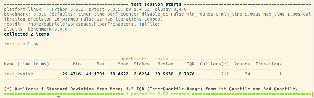
Figure 1.4 – Output from pytest
For each test collected, pytest-benchmark will execute the benchmark function several times and provide a statistic summary of its running time. The preceding output shown is very interesting as it shows how running times vary between runs.
In this example, the benchmark in test_evolve was run 34 times (Rounds column), its timings ranged between 29 and 41 milliseconds (ms) (Min and Max), and the Average and Median times were fairly similar at about 30 ms, which is actually very close to the best timing obtained. This example demonstrates how there can be substantial performance variability between runs and that, as opposed to taking timings with one-shot tools such as time, it is a good idea to run the program multiple times and record a representative value, such as the minimum or the median.
pytest-benchmark has many more features and options that can be used to take accurate timings and analyze the results. For more information, consult the documentation at http://pytest-benchmark.readthedocs.io/en/stable/usage.html.
Finding bottlenecks with cProfile
After assessing the correctness and timing of the execution time of the program, we are ready to identify the parts of the code that need to be tuned for performance. We typically aim to identify parts that are small compared to the size of the program.
Two profiling modules are available through the Python standard library, as outlined here:
- The profile module: This module is written in pure Python and adds significant overhead to the program execution. Its presence in the standard library is due to its vast platform support and the ease with which it can be extended.
- The cProfile module: This is the main profiling module, with an interface equivalent to
profile. It is written in C, has a small overhead, and is suitable as a general-purpose profiler.
The cProfile module can be used in three different ways, as follows:
- From the command line
- As a Python module
- With IPython
cProfile does not require any change in the source code and can be executed directly on an existing Python script or function. You can use cProfile from the command line in this way:
$ python -m cProfile simul.py
This will print a long output containing several profiling metrics of all of the functions called in the application. You can use the -s option to sort the output by a specific metric. In the following snippet, the output is sorted by the tottime metric, which will be described here:
$ python -m cProfile -s tottime simul.py
The data produced by cProfile can be saved in an output file by passing the -o option. The format that cProfile uses is readable by the stats module and other tools. The usage of the-o option is shown here:
$ python -m cProfile -o prof.out simul.py
The usage of cProfile as a Python module requires invoking the cProfile.run function in the following way:
    from simul import benchmark
    import cProfile
    cProfile.run("benchmark()")
You can also wrap a section of code between method calls of a cProfile.Profile object, as shown here:
    from simul import benchmark
    import cProfile
    pr = cProfile.Profile()
    pr.enable()
    benchmark()
    pr.disable()
    pr.print_stats()
cProfile can also be used interactively with IPython. The %prun magic command lets you profile an individual function call, as illustrated in the following screenshot:
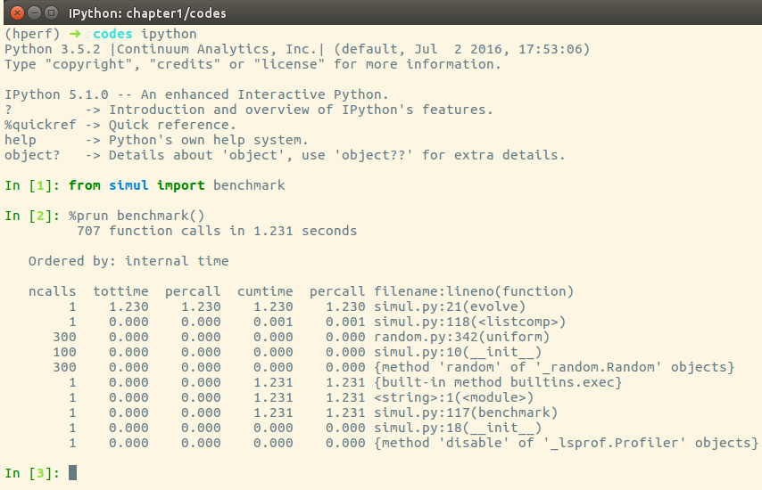
Figure 1.5 – Using cProfile within IPython
The cProfile output is divided into five columns, as follows:
ncalls: The number of times the function was called.tottime: The total time spent in the function without taking into account the calls to other functions.cumtime: The time spent in the function including other function calls.percall: The time spent for a single call of the function—this can be obtained by dividing the total or cumulative time by the number of calls.filename:lineno: The filename and corresponding line numbers. This information is not available when calling C extension modules.
The most important metric is tottime, the actual time spent in the function body excluding subcalls, which tells us exactly where the bottleneck is.
Unsurprisingly, the largest portion of time is spent in the evolve function. We can imagine that the loop is the section of the code that needs performance tuning. cProfile only provides information at the function level and does not tell us which specific statements are responsible for the bottleneck. Fortunately, as we will see in the next section, the line_profiler tool is capable of providing line-by-line information of the time spent in the function.
Analyzing the cProfile text output can be daunting for big programs with a lot of calls and subcalls. Some visual tools aid the task by improving navigation with an interactive, graphical interface.
Graphically analyzing profiling results
KCachegrind is a graphical user interface (GUI) useful for analyzing the profiling output emitted by cProfile.
KCachegrind is available in the Ubuntu 16.04 official repositories. The Qt port, QCacheGrind, can be downloaded for Windows from http://sourceforge.net/projects/qcachegrindwin/. Mac users can compile QCacheGrind using MacPorts (http://www.macports.org/) by following the instructions present in the blog post at http://blogs.perl.org/users/rurban/2013/04/install-kachegrind-on-macosx-with-ports.html.
KCachegrind can't directly read the output files produced by cProfile. Luckily, the pyprof2calltree third-party Python module is able to convert the cProfile output file into a format readable by KCachegrind.
You can install pyprof2calltree from the Python Package Index (PyPI) using the pip install pyprof2calltree command.
To best show the KCachegrind features, we will use another example with a more diversified structure. We define a recursive function, factorial, and two other functions that use factorial, named taylor_exp and taylor_sin. They represent the polynomial coefficients of the Taylor approximations of exp(x) and sin(x) and are illustrated in the following code snippet:
    def factorial(n):
        if n == 0:
            return 1.0
        else:
            return n * factorial(n-1)
    def taylor_exp(n):
        return [1.0/factorial(i) for i in range(n)]
    def taylor_sin(n):
        res = []
        for i in range(n):
            if i % 2 == 1:
               res.append((-1)**((i-1)/2)/
                   float(factorial(i)))
            else:
               res.append(0.0)
        return res
    def benchmark():
        taylor_exp(500)
        taylor_sin(500)
    if __name__ == '__main__':
        benchmark()
To access profile information, we first need to generate a cProfile output file, as follows:
$ python -m cProfile -o prof.out taylor.py
Then, we can convert the output file with pyprof2calltree and launch KCachegrind by running the following code:
$ pyprof2calltree -i prof.out -o prof.calltree
$ kcachegrind prof.calltree # or qcachegrind prof.calltree
The output is shown in the following screenshot:
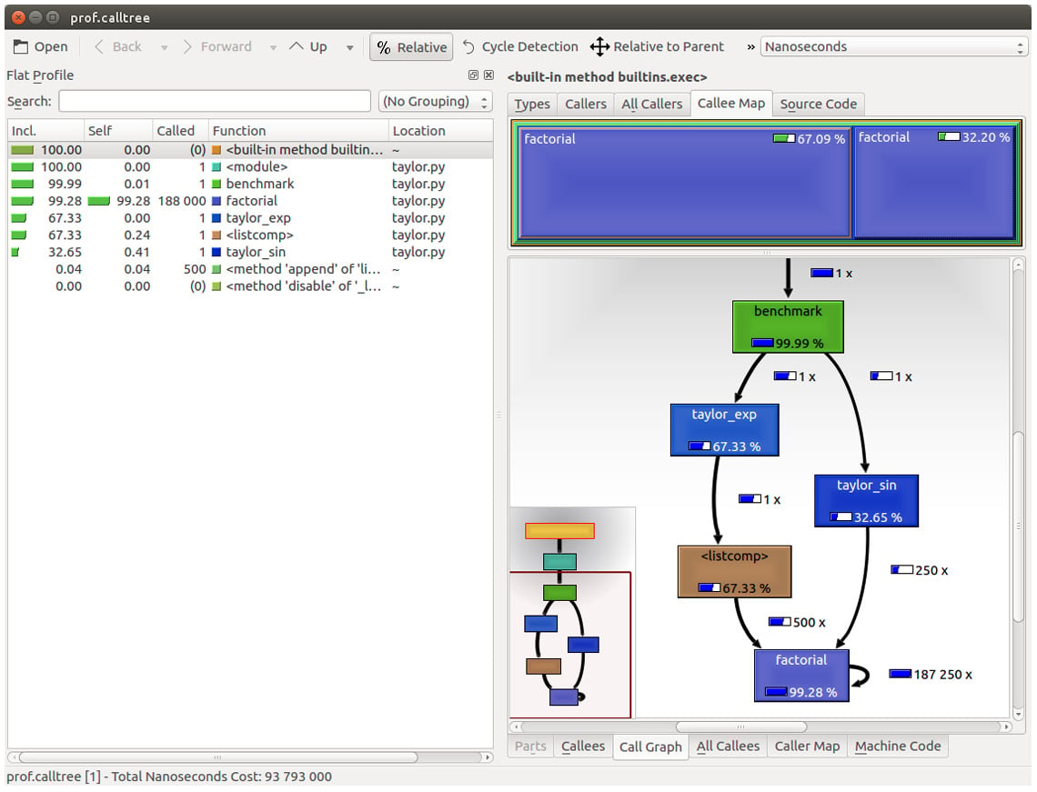
Figure 1.6 – Profiling output generated by pyprof2calltree and displayed by KCachegrind
The screenshot shows the KCachegrind UI. On the left, we have an output fairly similar to cProfile. The actual column names are slightly different: Incl. translates to the cProfile module's cumtime value and Self translates to tottime. The values are given in percentages by clicking on the Relative button on the menu bar. By clicking on the column headers, you can sort them by the corresponding property.
On the top right, a click on the Callee Map tab will display a diagram of the function costs. In the diagram shown in Figure 1.6, the time percentage spent by the function is proportional to the area of the rectangle. Rectangles can contain sub-rectangles that represent subcalls to other functions. In this case, we can easily see that there are two rectangles for the factorial function. The one on the left corresponds to the calls made by taylor_exp and the one on the right to the calls made by taylor_sin.
On the bottom right, you can display another diagram, a call graph, by clicking on the Call Graph tab. A call graph is a graphical representation of the calling relationship between the functions; each square represents a function and the arrows imply a calling relationship. For example, taylor_exp calls factorial 500 times, and taylor_sin calls factorial 250 times. KCachegrind also detects recursive calls: factorial calls itself 187250 times.
You can navigate to the Call Graph or the Callee Map tab by double-clicking on the rectangles; the interface will update accordingly, showing that the timing properties are relative to the selected function. For example, double-clicking on taylor_exp will cause the graph to change, showing only the contribution of taylor_exp to the total cost.
Gprof2Dot (https://github.com/jrfonseca/gprof2dot) is another popular tool used to produce call graphs. Starting from output files produced by one of the supported profilers, it will generate a .dot diagram representing a call graph.
Profiling line by line with line_profiler
Now that we know which function we have to optimize, we can use the line_profiler module that provides information on how time is spent in a line-by-line fashion. This is very useful in situations where it's difficult to determine which statements are costly. The line_profiler module is a third-party module that is available on PyPI and can be installed by following the instructions at https://github.com/rkern/line_profiler.
In order to use line_profiler, we need to apply a @profile decorator to the functions we intend to monitor. Note that you don't have to import the profile function from another module as it gets injected into the global namespace when running the kernprof.py profiling script. To produce profiling output for our program, we need to add the @profile decorator to the evolve function, as follows:
    @profile
    def evolve(self, dt):
        # code
The kernprof.py script will produce an output file and print the result of the profiling on the standard output. We should run the script with two options, as follows:
-lto use theline_profilerfunction-vto immediately print the results on screen
The usage of kernprof.py is illustrated in the following line of code:
$ kernprof.py -l -v simul.py
It is also possible to run the profiler in an IPython shell for interactive editing. You should first load the line_profiler extension that will provide the lprun magic command. Using that command, you can avoid adding the @profile decorator, as illustrated in the following screenshot:
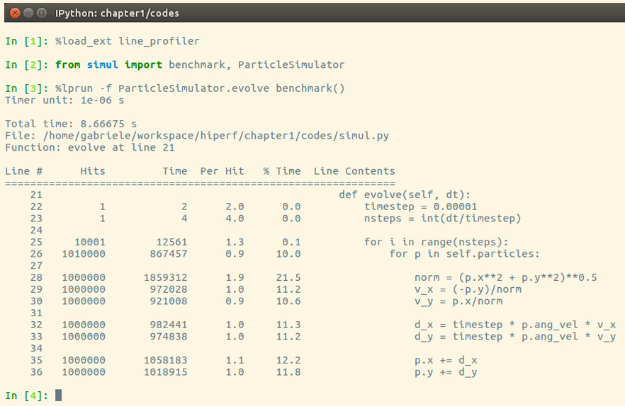
Figure 1.7 – Using line_profiler within IPython
The output is quite intuitive and is divided into six columns, as follows:
Line #: The number of the line that was runHits: The number of times that line was runTime: The execution time of the line in microseconds (Time)Per Hit: Time/hits% Time: Fraction of the total time spent executing that lineLine Contents: The content of the line
By looking at the % Time column, we can get a pretty good idea of where the time is spent. In this case, there are a few statements in the for loop body with a cost of around 10-20 percent each.
Optimizing our code
Now that we have identified where exactly our application is spending most of its time, we can make some changes and assess the resulting improvement in performance.
There are different ways to tune up our pure Python code. The way that typically produces the most significant results is to improve the algorithms used. In this case, instead of calculating the velocity and adding small steps, it will be more efficient (and correct, as it is not an approximation) to express the equations of motion in terms of radius, r, and angle, alpha, (instead of x and y), and then calculate the points on a circle using the following equation:
    x = r * cos(alpha)
    y = r * sin(alpha)
Another optimization method lies in minimizing the number of instructions. For example, we can precalculate the timestep * p.ang_vel factor that doesn't change with time. We can exchange the loop order (first, we iterate on particles, then we iterate on time steps) and put the calculation of the factor outside the loop on the particles.
The line-by-line profiling also showed that even simple assignment operations can take a considerable amount of time. For example, the following statement takes more than 10 percent of the total time:
v_x = (-p.y)/norm
We can improve the performance of the loop by reducing the number of assignment operations performed. To do that, we can avoid intermediate variables by rewriting the expression into a single, slightly more complex statement (note that the right-hand side gets evaluated completely before being assigned to the variables), as follows:
    p.x, p.y = p.x - t_x_ang*p.y/norm, p.y + t_x_ang *
    p.x/norm
This leads to the following code:
        def evolve_fast(self, dt):
            timestep = 0.00001
            nsteps = int(dt/timestep)
            # Loop order is changed
            for p in self.particles:
                t_x_ang = timestep * p.ang_vel
                for i in range(nsteps):
                    norm = (p.x**2 + p.y**2)**0.5
                    p.x, p.y = (p.x - t_x_ang * p.y/norm,
                        p.y + t_x_ang * p.x/norm)
After applying the changes, we should verify that the result is still the same by running our test. We can then compare the execution times using our benchmark, as follows:
$ time python simul.py # Performance Tuned
real    0m0.756s
user    0m0.714s
sys    0m0.036s
$ time python simul.py # Original
real    0m0.863s
user    0m0.831s
sys    0m0.028s
As you can see, we obtained only a modest increment in speed by making a pure Python micro-optimization.
Using the dis module
In this section, we will dig into the Python internals to estimate the performance of individual statements. In the CPython interpreter, Python code is first converted to an intermediate representation, the bytecode, and then executed by the Python interpreter.
To inspect how the code is converted to bytecode, we can use the dis Python module (dis stands for disassemble). Its usage is really simple; all we need to do is call the dis.dis function on the ParticleSimulator.evolve method, like this:
    import dis
    from simul import ParticleSimulator
    dis.dis(ParticleSimulator.evolve)
This will print, for each line in the function, a list of bytecode instructions. For example, the v_x = (-p.y)/norm statement is expanded in the following set of instructions:
    29           85 LOAD_FAST                5 (p)
                 88 LOAD_ATTR                4 (y)
                 91 UNARY_NEGATIVE
                 92 LOAD_FAST                6 (norm)
                 95 BINARY_TRUE_DIVIDE
                 96 STORE_FAST               7 (v_x)
LOAD_FAST loads a reference of the p variable onto the stack and LOAD_ATTR loads the y attribute of the item present on top of the stack. The other instructions, UNARY_NEGATIVE and BINARY_TRUE_DIVIDE, simply do arithmetic operations on top-of-stack items. Finally, the result is stored in v_x (STORE_FAST).
By analyzing the dis output, we can see that the first version of the loop produces 51 bytecode instructions, while the second gets converted into 35 instructions.
The dis module helps discover how the statements get converted and serves mainly as an exploration and learning tool of the Python bytecode representation. For a more comprehensive introduction and discussion on the Python bytecode, refer to the Further reading section at the end of this chapter.
To improve our performance even further, we can keep trying to figure out other approaches to reduce the number of instructions. It's clear, however, that this approach is ultimately limited by the speed of the Python interpreter, and it is probably not the right tool for the job. In the following chapters, we will see how to speed up interpreter-limited calculations by executing fast specialized versions written in a lower-level language (such as C or Fortran).
Profiling memory usage with memory_profiler
In some cases, high memory usage constitutes an issue. For example, if we want to handle a huge number of particles, we will incur a memory overhead due to the creation of many Particle instances.
The memory_profiler module summarizes, in a way similar to line_profiler, the memory usage of a process.
The memory_profiler package is also available on PyPI. You should also install the psutil module (https://github.com/giampaolo/psutil) as an optional dependency that will make memory_profiler considerably faster.
Just as with line_profiler, memory_profiler also requires the instrumentation of the source code by placing a @profile decorator on the function we intend to monitor. In our case, we want to analyze the benchmark function.
We can slightly change benchmark to instantiate a considerable amount (100000) of Particle instances and decrease the simulation time, as follows:
    def benchmark_memory():
        particles = [
                     Particle(uniform(-1.0, 1.0),
                              uniform(-1.0, 1.0),
                              uniform(-1.0, 1.0))
                      for i in range(100000)
            ]
        simulator = ParticleSimulator(particles)
        simulator.evolve(0.001)
We can use memory_profiler from an IPython shell through the %mprun magic command, as shown in the following screenshot:
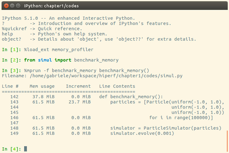
Figure 1.8 – Output from memory_profiler
It is possible to run memory_profiler from the shell using the mprof run command after adding the @profile decorator.
From the Increment column, we can see that 100,000 Particle objects take 23.7 MiB of memory.
1 mebibyte (MiB) is equivalent to 1,048,576 bytes. It is different from 1 megabyte (MB), which is equivalent to 1,000,000 bytes.
We can use __slots__ on the Particle class to reduce its memory footprint. This feature saves some memory by avoiding storing the variables of the instance in an internal dictionary. This strategy, however, has a small limitation—it prevents the addition of attributes other than the ones specified in __slots__. You can see this feature in use in the following code snippet:
    class Particle:
        __slots__ = ('x', 'y', 'ang_vel')
        def __init__(self, x, y, ang_vel):
            self.x = x
            self.y = y
            self.ang_vel = ang_vel
We can now rerun our benchmark to assess the change in memory consumption. The result is displayed in the following screenshot:
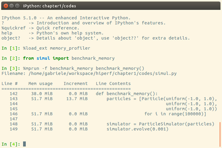
Figure 1.9 – Improvement in memory consumption
By rewriting the Particle class using __slots__, we can save about 10 MiB of memory.
Summary
In this chapter, we introduced the basic principles of optimization and applied those principles to a test application. When optimizing an application, the first thing to do is test and identify the bottlenecks in the application. We saw how to write and time a benchmark using the time Unix command, the Python timeit module, and the full-fledged pytest-benchmark package. We learned how to profile our application using cProfile, line_profiler, and memory_profiler, and how to analyze and navigate the profiling data graphically with KCachegrind.
Speed is undoubtedly an important component of any modern software. The techniques we have learned in this chapter will allow you to systematically tackle the problem of making your Python programs more efficient from different angles. Further, we have seen that these tasks can take advantage of Python built-in/native packages and do not require any special external tools.
In the next chapter, we will explore how to improve performance using algorithms and data structures available in the Python standard library. We will cover scaling and sample usage of several data structures, and learn techniques such as caching and memorization. We will also introduce Big O notation, which is a common computer science tool to analyze the running time of algorithms and data structures.
Questions
- Arrange the following three items in order of importance when building a software application: correctness (the program does what it is supposed to do), efficiency (the program is optimized in speed and memory management), and functionality (the program runs).
- How could
assertstatements be used in Python to check for the correctness of a program? - What is a benchmark in the context of optimizing a software program?
- How could
timeitmagic commands be used in Python to estimate the speed of a piece of code? - List three different types of information that are recorded and returned by
cProfile(included as output columns) in the context of profiling a program. - On a high level, what is the role of the
dismodule in optimization? - In the
exercise.pyfile, we write a simple function,close(), that checks whether a pair of particles are close to each other (with 1e-5 tolerance). Inbenchmark(), we randomly initialize two particles and callclose()after running the simulation. Make a guess of what takes most of the execution time inclose(), and profile the function viabenchmark()usingcProfile; does the result confirm your guess?
Further reading
- Profilers in Python: https://docs.python.org/3/library/profile.html
- Using PyCharm's profiler: https://www.jetbrains.com/help/pycharm/profiler.html
- A beginner-friendly introduction to bytecode in Python: https://opensource.com/article/18/4/introduction-python-bytecode
